Introduction
Hello! In our last lesson, we established the concept of the canonical link function, the "natural" connection that equates the model's linear predictor () with the distribution's natural parameter (). We identified the identity, log, and logit links as the canonical choices for the Normal, Poisson, and Binomial distributions, respectively.
While canonical links are mathematically elegant and the default choice, they are not the only choice. The real world doesn't always conform to the neatest mathematical form. This lesson tackles the question: what other options do we have, and when should we use them?
Our goal is to distinguish between canonical and non-canonical link functions. We will focus on the most common practical choice you'll face—selecting a link for binary outcomes—by comparing the canonical logit link to its main competitor, the probit link. We'll explore the key trade-offs to consider when making this choice, aligning with your goal of understanding how these methods work functionally and when one is preferred over another.
Canonical vs. Non-Canonical Links
As a quick recap, a link function must be a monotonic and differentiable function. The canonical link is special because it makes the linear predictor equal to the natural parameter of the response distribution in its exponential family form ().
Any other valid link function is called a non-canonical link.
So, why would we ever deviate from the canonical choice? While canonical links have desirable statistical properties that can simplify estimation, there is no guarantee that they provide the best description of the relationship in your specific dataset. The primary goal of modeling is to find a function that accurately reflects the underlying data-generating process.
To see this distinction in action, let's watch a brief segment that introduces the idea of non-canonical links.
GLM Link Function, and Canonical Links
In the video 'GLM Link Function, and Canonical Links' from Stats4Everyone, which we viewed parts of in the last lesson, the presenter concludes by mentioning that other links exist and are sometimes better.
Please watch from 07:40 to 09:18. This section highlights that canonical links are not the only option and introduces probit and complementary log-log as popular non-canonical choices for binomial data.
The key takeaway is that we can, and sometimes should, test different links to see which provides a better fit for our data.
A Case Study: Link Functions for Binary Outcomes
The choice between link functions is most prominent when modeling binary (0/1) or proportional outcomes with the binomial distribution. As you know, the goal is to model the probability of success, , which is bounded between 0 and 1. The link function's job is to map this (0, 1) interval onto the entire real number line (-, +), which is the range of the linear predictor .
Any function that produces an "S"-shaped (sigmoidal) curve can accomplish this. The canonical link for the binomial distribution is the logit link, but several non-canonical alternatives exist.
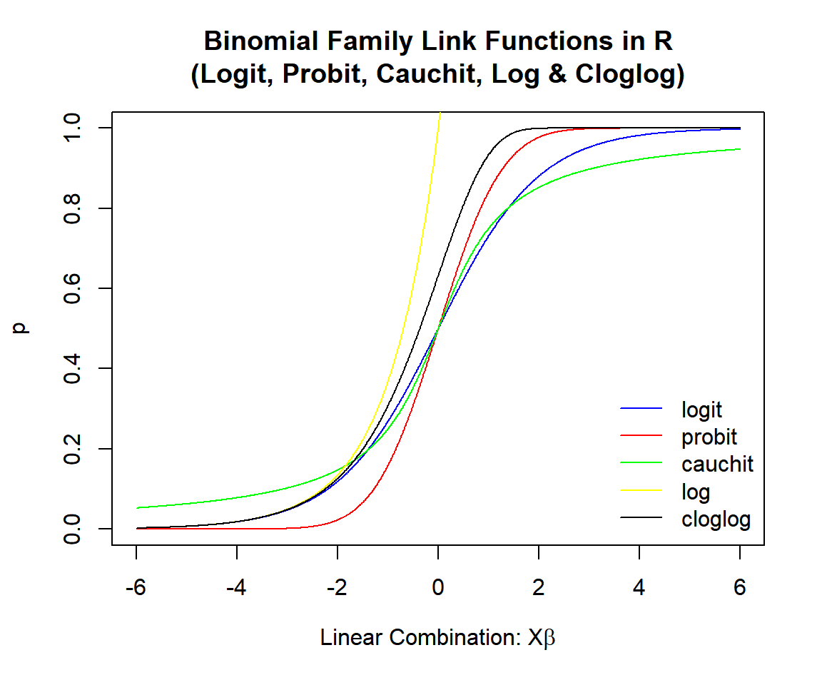
The two most widely used links for binary data are the logit and probit links. Let's explore them in detail.
Deep Dive: The Logit vs. Probit Links
Understanding the difference between logit and probit models is crucial in applied data science. The following video provides an excellent and intuitive introduction to both.
Discrete choice models - introduction to logit and probit
This video from Ben Lambert, 'Discrete choice models - introduction to logit and probit,' clearly explains the motivation for both models and their mathematical underpinnings.
Please watch the entire video (00:00 - 09:47). Pay attention to: Why a non-linear transformation is needed for probabilities. The mathematical form of the logit function and how it's derived from the logistic distribution. The form of the probit function and its connection to the standard normal distribution's cumulative distribution function (CDF). The comparison of their key properties and the reasons for choosing one over the other.
To summarize and formalize the points from the video:
The Logit Link (Canonical)
- Form:
- Underlying Distribution: It is derived from the CDF of the logistic distribution.
- Interpretation: This is its main advantage. Since is the odds of success, the logit link models the log-odds of the outcome as a linear function of the predictors. This means model coefficients can be exponentiated to get odds ratios, which are highly interpretable.
The Probit Link (Non-Canonical)
- Form: , where is the inverse CDF of the standard normal distribution.
- Underlying Distribution: It is derived from the CDF of the standard normal distribution.
- Interpretation: A probit model assumes that there is an unobserved (latent) continuous variable that follows a normal distribution. The binary outcome we observe depends on whether this latent variable crosses a certain threshold. The coefficients are on the scale of this latent variable (in standard deviations), which is less intuitive than odds ratios.
Other Notable Non-Canonical Links
While logit and probit are the most common, other links are useful in specific scenarios, particularly when the relationship is asymmetric.
[PDF] Chapter 3 Generalized Linear Models (GLM)
The following document from the University of Chicago provides a concise summary of several link functions for binomial data.
Please read the sections titled 'Complementary Log-Log Models,' 'Log-log Models,' and 'Link Functions' (pages 15-17). Focus on how the text describes the asymmetric behavior of the complementary log-log and log-log links.
-
Complementary Log-Log (cloglog):
- Form:
- Use Case: This link is asymmetric. It's appropriate when the probability of success approaches 1 quickly but approaches 0 slowly. This is common in survival analysis where the probability of an event (like equipment failure) is low for a long time and then rises sharply.
-
Log-Log:
- Form:
- Use Case: This link has the opposite asymmetry of the cloglog link. The probability approaches 0 quickly but approaches 1 slowly.
The Trade-Offs: How to Choose Your Link
You now know what the main canonical and non-canonical links are. So, how do you choose? The decision involves balancing interpretability, theoretical assumptions, and model fit.
[PDF] Chapter 3 Generalized Linear Models (GLM)
The same document provides a practical guide on this choice.
Now, read the section 'How to Choose a Link Function?' on page 21. It directly addresses the practical trade-offs between logit and probit models.
Here is a summary of the key trade-offs:
| Criterion | Logit (Canonical) | Probit (Non-Canonical) | The Verdict |
|---|---|---|---|
| Interpretability | Excellent. Coefficients directly relate to log-odds ratios, which are easy to explain. | Poor. Coefficients relate to a latent normal variable and are not directly interpretable in a practical sense. | Winner: Logit. This is the primary reason for its popularity in many fields. |
| Model Fit | Logit and Probit curves are very similar. The logistic distribution has slightly "heavier" tails than the normal distribution. | For most datasets, the fitted probabilities and model conclusions will be nearly identical. | Usually a draw. Differences only appear with very large datasets or where data is concentrated in the extreme tails of the distribution. |
| Theoretical Properties | Possesses special properties due to being canonical. For example, it allows for the formation of conditional logistic regression models for matched data, a topic we will cover later. | Does not have the same sufficiency properties, so some advanced models (like conditional probit) are not possible. | Winner: Logit. Its canonical status gives it more flexibility for certain advanced modeling techniques. |
| Underlying Theory | Assumes the log-odds of the outcome is a linear combination of predictors. | Assumes a normally distributed latent variable drives the outcome. This may be theoretically appealing in fields like econometrics. | Depends on your field and theoretical preference. |
For more on the theoretical advantages of canonical links, the following resource provides a key insight.
What is the difference between a 'link function' and a 'canonical link ...'
This Stack Exchange answer offers a concise but important point about a theoretical property of the canonical link.
Read the short answer by the user 'StasK'. The key takeaway is that the canonical logit link allows for certain models (like conditional logit) that are not possible with the non-canonical probit link due to properties of statistical sufficiency.
Conclusion
In this lesson, we moved beyond the default choice of canonical links and explored the world of non-canonical alternatives. You learned that while canonical links offer mathematical convenience and desirable properties, non-canonical links provide the flexibility to better capture the true nature of your data.
Key Takeaways:
- A non-canonical link is any valid link function that is not the canonical one for a given distribution.
- For binary data, the main choice is between the canonical logit link and the non-canonical probit link.
- The logit link is generally preferred due to the high interpretability of its coefficients as odds ratios.
- The probit link assumes an underlying normally distributed latent variable and is common in fields like econometrics, but its coefficients are difficult to interpret.
- In practice, logit and probit models often yield very similar results. The choice is often driven by the need for interpretability or conventions within a specific field.
- Other non-canonical links, like complementary log-log, are useful for modeling asymmetric relationships.
Preview of the Next Lesson:
We have now covered all three components of a GLM: the Random component (distribution), the Systematic component (linear predictor), and the Link function. Now we can start using them! In the next lesson, "Inference and Model Assessment for GLMs," we will begin to explore how to evaluate how well a GLM fits the data. We'll start by defining the concept of deviance, which is the core metric for measuring goodness of fit in the GLM framework.