Introduction
Hello! In our previous lesson, we established a critical rule: the standard Pearson chi-square test is unsuitable for paired data because it violates the core assumption of independent observations. We saw that in a "before-and-after" study, the two measurements from the same person are inherently linked, and using a test that assumes they aren't leads to invalid conclusions.
This lesson provides the solution to that problem. We will explore the McNemar test, which is specifically designed to analyze changes in paired binary outcomes. By the end of this lesson, you will be able to describe how the McNemar test works, what its hypotheses are, how to interpret its results, and when it is the appropriate tool for your analysis.
1. The Core Idea: Focusing on What Changed
The genius of the McNemar test is its simplicity. Instead of getting bogged down by all the data, it focuses only on the subjects who showed a change. These are the only subjects who provide information about whether the intervention or time-lapse had an effect.
To begin, let's get a clear definition of McNemar's test and understand its logic.
McNemar’s Test: The Hidden Gem for Paired Binary Data
This article provides an excellent introduction to McNemar's test, explaining why it's designed for paired data and what it actually measures.
Please read the sections 'What Is McNemar’s Test?', 'Why Paired Data Matters', and 'What McNemar’s Test Actually Tests'. Focus on how the test uses a 2x2 table but only considers the 'off-diagonal' cells.
2. Concordant vs. Discordant Pairs
The reading you just completed introduced the idea of focusing on disagreements. In statistical terms, we classify each pair of observations as either concordant (the outcomes agree) or discordant (the outcomes disagree).
Let's use a typical pre-test/post-test scenario to define these terms:
- Concordant Pairs: Individuals whose outcome did not change.
- They answered "No" on the pre-test and "No" on the post-test.
- They answered "Yes" on the pre-test and "Yes" on the post-test.
- Discordant Pairs: Individuals whose outcome did change.
- They answered "Yes" on the pre-test but "No" on the post-test.
- They answered "No" on the pre-test but "Yes" on the post-test.
The McNemar test completely ignores the concordant pairs. Why? Because a person who started at "Yes" and ended at "Yes" tells us nothing about the effectiveness of an intervention meant to cause change. The only information about a potential shift comes from those who switched categories.
3. The McNemar Test: Hypotheses and Statistic
The test works by comparing the number of subjects who changed in one direction to the number who changed in the opposite direction.
Let's represent this in a 2x2 contingency table. Note the specific meaning of each cell:
| Post-Test: Yes | Post-Test: No | |
|---|---|---|
| Pre-Test: Yes | a | b |
| Pre-Test: No | c | d |
- Cell a: Yes -> Yes (Concordant)
- Cell b: Yes -> No (Discordant)
- Cell c: No -> Yes (Discordant)
- Cell d: No -> No (Concordant)
The McNemar test focuses only on cells b and c.
Hypotheses
The question McNemar's test asks is: "Is the number of people who switched from Yes to No (cell b) significantly different from the number of people who switched from No to Yes (cell c)?"
- Null Hypothesis (H₀): There is no significant change in proportions. The probability of switching from Yes to No is equal to the probability of switching from No to Yes. In terms of our table, the expected counts in cells b and c are equal.
- Alternative Hypothesis (H₁): There is a significant change in proportions. The probabilities of switching in each direction are not equal.
The Test Statistic
To test this, we use a statistic that follows the chi-squared distribution with 1 degree of freedom.

As shown in the image, the formula is:
Where b and c are the counts of the two discordant pairs. You can see how the formula directly compares the counts in the two cells of interest. If b and c are very similar, the numerator (b-c)^2 will be small, leading to a small value and a large p-value (fail to reject H₀). If b and c are very different, the numerator will be large, leading to a large value and a small p-value (reject H₀).
For small sample sizes (when b + c is less than ~25), a "continuity correction" is often applied to make the chi-squared approximation more accurate. The formula becomes:
You don't need to memorize this, but it's good to know it exists, as most software will apply it by default.
4. A Practical Walkthrough
Let's see this in action. The best way to build a functional understanding is to see the calculation done step-by-step.
This video demonstrates how to perform the McNemar test manually in Excel. This approach is excellent for revealing the test's inner workings, as it forces us to identify and count the discordant pairs before applying the formula.
Watch from 04:03 to 07:06. The presenter has already identified subjects who changed. Pay attention to how he first counts the two 'change' groups (the discordant pairs) and then plugs these counts directly into the test statistic formula.
The video shows exactly the logic we've discussed:
- Isolate the subjects who changed.
- Count the number who changed from A to B (e.g., Support -> No Support).
- Count the number who changed from B to A (e.g., No Support -> Support).
- Plug these two counts into the McNemar formula to get the test statistic.
5. Interpreting Software Output
In practice, you will use statistical software. The output will typically give you both the contingency table and the final test results.
Let's look at a sample output for a study measuring responses before and after an advertisement.
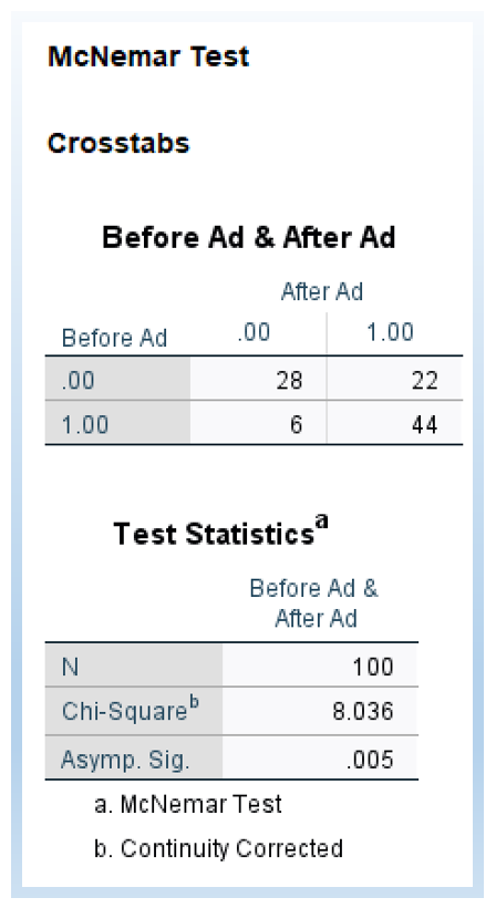
Here is how to interpret this output:
- Identify the Discordant Pairs: Look at the off-diagonal cells.
- b: Count of people who responded 'Yes' (1.00) before and 'No' (0.00) after = 6.
- c: Count of people who responded 'No' (0.00) before and 'Yes' (1.00) after = 22.
- Check the Test Statistic: The output gives a Chi-Square value of 8.036. The footnote tells us this is from the McNemar test. (This value was calculated using the continuity correction: ).
- Evaluate the p-value: The significance ("Asymp. Sig.") is .005.
- Make a Conclusion: Since the p-value (0.005) is less than the standard alpha level of 0.05, we reject the null hypothesis. We conclude that there was a statistically significant change in responses after viewing the ad. Specifically, significantly more people switched from "No" to "Yes" (22 people) than from "Yes" to "No" (6 people).
Conclusion
In this lesson, we introduced the McNemar test as the correct tool for analyzing pre-post changes in paired 2x2 tables. You now have a functional understanding of how it works and what it tells you.
Key Takeaways:
- The McNemar test is used for paired, dichotomous (binary) data.
- It tests whether there is a significant change in proportions between the two paired measurements.
- Its logic is based on comparing the discordant pairs—those who changed from Yes to No versus those who changed from No to Yes.
- The concordant pairs (Yes to Yes, No to No) are ignored as they provide no information about change.
- A low p-value indicates that the change observed (the difference between the two types of discordant pairs) is statistically significant.
Preview of the Next Lesson:
The McNemar test is powerful, but it's limited to 2x2 tables. What if your categorical variable has more than two levels? For example, what if you were measuring opinions as "Agree," "Neutral," and "Disagree" before and after an event? In the next lesson, we will learn about the Stuart-Maxwell test, which is a generalization of the McNemar test for analyzing k×k tables.