Introduction
Hello! In our last lesson, you learned the fundamental principles of the McNemar test. We established that it is the correct statistical tool for analyzing paired, binary data, such as in a "before-and-after" study. You saw that its logic is to test for a significant difference in the "discordant pairs"—the subjects who changed their response between the two measurements.
This lesson transitions from theory to practice. Our goal is to solidify your functional understanding by applying the McNemar test to a realistic dataset. You will learn how to:
- Set up the data correctly in a contingency table.
- Use statistical software to perform the test.
- Interpret the complete output, including not just the p-value but also the direction and magnitude of the change.
By the end of this lesson, you will be able to confidently apply the McNemar test to a problem and articulate a meaningful conclusion based on its results.
1. A Practical Scenario: The Rain Barrel Workshop
Let's ground our learning in a common scenario. A local environmental group holds a workshop to encourage residents to install rain barrels. To measure the workshop's effectiveness, they survey attendees before and after, asking a simple "Yes/No" question: "Are you planning to install a rain barrel?"
The collected data from 46 attendees is summarized in the following 2x2 contingency table:
| After: Yes | After: No | Row Total | |
|---|---|---|---|
| Before: Yes | 9 | 5 | 14 |
| Before: No | 17 | 15 | 32 |
| Column Total | 26 | 20 | 46 |
Before we run any tests, let's interpret the table:
- Concordant pairs (no change): 9 people said "Yes" both times, and 15 people said "No" both times. These 24 people provide no information about the workshop's impact on changing minds.
- Discordant pairs (change): These are the people we care about for this analysis.
- Cell b: 5 people who initially planned to install a rain barrel changed their minds to "No".
- Cell c: 17 people who did not initially plan to install one changed their minds to "Yes".
The question for the McNemar test is: Is the shift from "No" to "Yes" (17 people) significantly greater than the shift from "Yes" to "No" (5 people)?
2. Performing the Test with Statistical Software
In a real data science workflow, you would use software like SPSS, R, or Python to perform this test. Let's see how it's done.
Walkthrough with SPSS
This video provides a clear, step-by-step demonstration of running and interpreting the McNemar test in SPSS, a common statistical package.
Performing the McNemar Test in SPSS
This video from Dr. Todd Grande will walk you through performing a McNemar test. Please focus on the first method shown, using the 'Crosstabs' function, as it provides the most useful output.
Watch the video from 03:00 to 05:52. Pay close attention to how the 'Before' and 'After' variables are placed into the rows and columns and how to read the Crosstabulation table and the Chi-Square Tests table to find the p-value.
The video reinforces the process: set up the paired variables, run the analysis, and locate the contingency table and the p-value in the output. The example in the video shows a significant result (p = .002), indicating a real change in substance use status.
Implementation in R and Python
For your data science work, you'll likely use a programming language. The implementation is straightforward.
McNemar’s Test: The Hidden Gem for Paired Binary Data
This resource, 'McNemar's Test: The Hidden Gem for Paired Binary Data', provides clean code examples for both Python and R.
Briefly review the section 'In Code'. You don't need to run it now, but notice how the 2x2 table is defined as a matrix or array, and then passed to a single function (mcnemar in Python, mcnemar.test in R).
As you can see, the process in code mirrors the logic: you first structure your data into the 2x2 contingency table of counts, then you apply the test function.
3. Interpreting the Full Story: Significance, Direction, and Effect Size
Running the test is just the first step. A full interpretation requires three components. Let's use our rain barrel example.
Using the mcnemar.test() function in R on our rain barrel data gives the following output (as seen in the R Handbook resource):
McNemar's Chi-squared test with continuity correction

data:  Matrix.1
McNemar's chi-squared = 5.5, df = 1, p-value = 0.01902
Let's break this down.
a) Statistical Significance (The p-value)
- Result: The p-value is 0.019.
- Conclusion: Since this value is less than the standard alpha level of 0.05, we reject the null hypothesis. This tells us that the change we observed is statistically significant; it is unlikely to be due to random chance.
b) Direction of Change
The p-value only tells us that a change occurred. To understand the nature of the change, we must look back at our discordant cells:
-
b (Yes -> No): 5 people
-
c (No -> Yes): 17 people
-
Conclusion: Significantly more people were persuaded to install a rain barrel (switched from No to Yes) than were dissuaded (switched from Yes to No). The workshop had a positive effect on intentions.
c) Effect Size (Magnitude of Change)
How large was this effect? Just because it's statistically significant doesn't mean it's practically important. For McNemar's test, the odds ratio (OR) is an excellent and intuitive measure of effect size.
It's calculated simply as the ratio of the two discordant cell counts: or . We typically put the larger number in the numerator so the OR is > 1.
For our data:
- Interpretation: The odds of a person switching their answer from "No" to "Yes" were 3.4 times greater than the odds of switching from "Yes" to "No". This indicates a strong, meaningful effect.
To help interpret these values, you can refer to established guidelines.
McNemar Test and Tests for Paired Nominal Data - R Handbook
The 'R Handbook' resource provides a helpful table for interpreting effect sizes for McNemar's test, including the odds ratio.
Read the first few paragraphs of the 'Effect size' section, up to and including the interpretation table. Note the cutoffs for small, medium, and large effects for the Odds Ratio.
According to the table in the resource, an odds ratio of 3.4 () is considered a large effect.
4. A Note on Assumptions
McNemar's test is robust, but there is one main consideration, as mentioned in the video you watched and the R Handbook resource:
- Sample Size: The chi-squared approximation works best when the number of discordant pairs (
b + c) is not too small. A common rule of thumb is thatb + cshould be at least 10. In our example,b + c = 5 + 17 = 22, so we are fine. If the sum is very small, an "exact" version of the test (based on the binomial distribution) is preferred, which most software can perform.
Exercise: Check Your Understanding
Let's apply what you've learned. A political campaign runs a TV ad and wants to know if it changed voters' opinions of their candidate. They survey 100 voters before and after the ad.
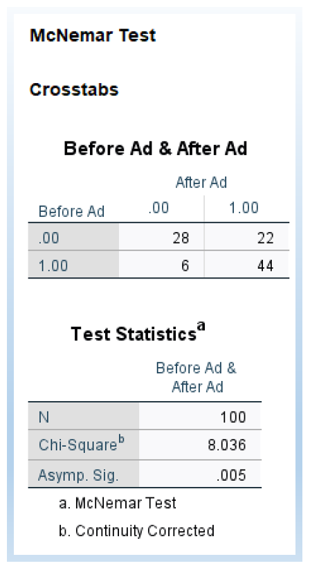
Based on the output in the image, answer the following questions:
- How many voters changed their opinion from "No" (coded as 0) to "Yes" (coded as 1) after seeing the ad?
- How many voters changed their opinion from "Yes" to "No"?
- What is the p-value for the McNemar test?
- Based on the p-value and the direction of change, what is your overall conclusion about the ad's effectiveness?
Answer
- 22 voters changed from "No" to "Yes" (bottom-left cell).
- 6 voters changed from "Yes" to "No" (top-right cell).
- The p-value is 0.005.
- Conclusion: Since the p-value (0.005) is less than 0.05, we reject the null hypothesis. There was a statistically significant change in opinion. Specifically, significantly more voters were persuaded by the ad (switching from No to Yes) than were dissuaded by it.
Conclusion
In this lesson, you moved from the theory of the McNemar test to its practical application. You learned how to take a real-world problem, structure the data, perform the test, and, most importantly, construct a comprehensive interpretation.
Key Takeaways:
- A full interpretation of a McNemar test includes the p-value (for statistical significance), the direction of change (by comparing discordant cells
bandc), and the effect size (often an odds ratio) to gauge the magnitude of the change. - The test is easily performed in statistical software or programming languages by first creating a 2x2 contingency table of counts.
- An odds ratio of
c/btells you how many times more likely a subject was to change in one direction compared to the other.
Preview of the Next Lesson:
The McNemar test is perfect for 2x2 tables. But what if your paired data isn't binary? For example, what if you measured satisfaction as "Low," "Medium," and "High" before and after a service change? For these situations, we need a more general tool. In the next lesson, we will explore the Stuart-Maxwell test, which extends the logic of McNemar's test to handle k×k tables.