Introduction
Hello! In our last few lessons, we've built a solid theoretical foundation for testing independence in contingency tables. We've explored:
- The logic of the Pearson chi-square test, which compares observed counts to expected counts.
- The principle of Fisher's exact test, which calculates exact probabilities for small samples.
- The general framework of permutation tests, which use shuffling to create an empirical null distribution.
Today, we shift from theory to practice. This lesson is all about application. You will learn how to perform these three tests using statistical software, interpret the output correctly, and report your findings in a clear and standard way. Crucially, we'll establish a decision-making framework so you'll know precisely which test is most appropriate for a given situation.
By the end of this lesson, you will be able to confidently apply chi-square, Fisher's exact, and permutation-based tests to real data and draw meaningful conclusions.
1. The Pearson Chi-Square Test in Practice
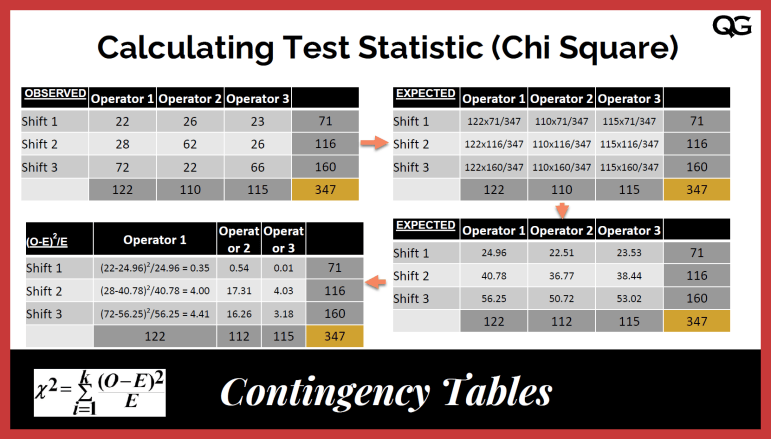
Let's start with the most common test for independence: the Pearson chi-square test. As a quick refresher, the test statistic, , quantifies the total difference between the observed counts in your table and the counts you would expect if the null hypothesis of no association were true.
Now, let's see how to apply this to a real dataset.
An Example: Mites and Plant Disease
We'll use an example from one of our resources involving an experiment on cotton plants. Researchers wanted to know if a prior infestation of spider mites would induce resistance to a fungal disease called Wilt.
The data is summarized in this 2x2 contingency table:
| Treatment | Wilt | No Wilt | Total |
|---|---|---|---|
| Mites | 9 | 17 | 26 |
| No Mites | 19 | 2 | 21 |
| Total | 28 | 19 | 47 |
The research question is: Is there a statistically significant association between mite treatment and the incidence of Wilt disease?
- Null Hypothesis (H₀): Mite treatment and the incidence of Wilt are independent. The proportion of plants that get Wilt is the same for both the treated and untreated groups.
- Alternative Hypothesis (Hₐ): Mite treatment and the incidence of Wilt are not independent.
Applying the Test
Instead of calculating the statistic by hand, we use software. The following resource shows how this is done in R and provides the output we need to interpret.
Chapter 11 Contingency Tables | Introduction to Statistical ...
Let's read a section from 'Chapter 11: Contingency Tables'. This will show us how to perform the chi-square test in R and how to extract and interpret the key results.
Please read the section titled '11.2 Hypothesis Testing'. Start from the beginning of this section and read down to where the text says 'We see that the p-value is 0.0188...'. Focus on how the chisq.test() function is used and what the output X-squared, df, and p-value represent.
Interpreting and Reporting the Results
As you saw in the reading, the R command chisq.test(table, correct=FALSE) gives us the key pieces of information. For the Mites data, the output is: X-squared = 7.2037, df = 1, p-value = 0.007275.
Here's how to break that down:
X-squared = 7.2037: This is the calculated chi-square statistic. It's a measure of how far our observed data deviates from the null hypothesis. A larger value suggests a greater deviation.df = 1: These are the degrees of freedom. For a contingency table, this is calculated as . For our 2x2 table, it's . The degrees of freedom determine the specific shape of the chi-square distribution we compare our statistic against.p-value = 0.007275: This is the probability of observing a chi-square statistic as large as 7.2037 (or larger) if the null hypothesis were true.
Since our p-value (0.0073) is less than the conventional significance level of , we reject the null hypothesis.
How to Report the Finding:
When reporting your results, you should always include the test statistic, degrees of freedom, p-value, and a clear statement of your conclusion in the context of the problem.
A Pearson's chi-square test was conducted to examine the relationship between mite treatment and the incidence of Wilt disease. The results indicated a significant association between the two variables, , . Plants that were not treated with mites were more likely to develop Wilt disease compared to those that were.
2. When Assumptions Fail: Fisher's and Permutation Tests
The chi-square test is an approximation that works well when sample sizes are large. Its primary assumption is that all expected cell counts should be greater than 5. When this assumption is violated, the calculated p-value may not be accurate.
This is a critical point for your functional understanding: you must always check the expected counts before trusting a chi-square result.

When you encounter this situation, you have two excellent alternatives.
2.1. Fisher's Exact Test: The Gold Standard for 2x2 Tables
As we've discussed, Fisher's Exact Test calculates the exact probability of observing the data, so it doesn't rely on the large-sample approximation. It is the preferred method for 2x2 tables with small expected counts.
Applying the Test:
Let's look at the resource below to see how to perform Fisher's test.
[PDF] Fall 2020 11. Chi Square Tests (plus Fisher's Exact Test)
This document, 'Chi Square Tests (plus Fisher's Exact Test)', explains when and how to apply Fisher's test. We will focus on the practical R code and interpretation.
Please read section '5b. Fisher's Exact Test'. Skim the initial hypothesis setup (which is the same as the chi-square test) and focus on the R code block on page 23. Notice the function is fisher.test() and its output includes a p-value and an odds ratio.
Interpreting and Reporting:
The output of fisher.test() gives you a p-value directly. For example, if we ran it on a dataset and got p-value = 0.021, we would conclude there is a significant association. The output also provides an odds ratio, a measure of association we studied earlier, which is very useful for interpretation.
How to Report the Finding:
Due to small expected cell counts, Fisher's exact test was used to examine the relationship between Variable A and Variable B. The test revealed a significant association between the variables (p = .021).
2.2. The Permutation Test: A Flexible Alternative
What if your table is larger than 2x2 and you have small expected counts? Fisher's test becomes computationally complex for large tables. This is where the permutation test we learned about in the last lesson becomes extremely useful. It provides a robust p-value without relying on the chi-square distribution's assumptions.
Applying the Test:
Fortunately, performing a permutation test in R is very simple. We use the same chisq.test function but add an argument to tell it to simulate the p-value by shuffling the data.
Chapter 11 Contingency Tables | Introduction to Statistical ...
Let's return to the 'Chapter 11: Contingency Tables' resource. It demonstrates how to enable the permutation option within the standard chi-square test function.
In the same section as before ('11.2 Hypothesis Testing'), find the paragraph that starts with 'As usual, it is pretty annoying to have to program the permutation test ourselves.' Read about the simulate.p.value=TRUE option and look at the corresponding R code and output.
Interpreting and Reporting:
The output will look similar to the standard test, but the p-value is derived from thousands of random shuffles. For the Mites data, the simulated p-value was 0.0148.
How to Report the Finding:
A chi-square test of independence with a simulated p-value based on 10,000 permutations was conducted... The result was significant (, simulated p = .015), indicating an association between mite treatment and Wilt disease.
3. A Decision Framework: Choosing the Right Test
You now have three tools. Here is a simple framework to help you choose the right one every time.
-
Construct your contingency table and calculate the expected counts for each cell.
- Expected Count =
-
Check the expected counts against the > 5 rule.
-
If all expected counts are > 5:
- The Pearson chi-square test is reliable and appropriate. Use
chisq.test().
- The Pearson chi-square test is reliable and appropriate. Use
-
If one or more expected counts are ≤ 5:
- Is the table 2x2?
- Yes -> Use Fisher's Exact Test. It is the most powerful and exact method in this scenario. Use
fisher.test().
- Yes -> Use Fisher's Exact Test. It is the most powerful and exact method in this scenario. Use
- Is the table larger than 2x2?
- Yes -> Use the chi-square test with permutation. It provides a reliable p-value when the theoretical distribution is not a good fit. Use
chisq.test(..., simulate.p.value=TRUE).
- Yes -> Use the chi-square test with permutation. It provides a reliable p-value when the theoretical distribution is not a good fit. Use
- Is the table 2x2?
-
This framework ensures your analysis is always statistically sound.
4. A Complete Example: R x C Table
Let's apply this framework to a larger table. The following example investigates the relationship between race and marital status using survey data. This is a 2x4 table.
Chapter 11 Contingency Tables | Introduction to Statistical ...
Finally, let's work through a full example with a larger table from 'Chapter 11: Contingency Tables'. This will consolidate everything we've learned.
Please read section '11.3 RxC tables'. Follow the example on the relationship between race and marriage status. Pay attention to: The visualization of the data. The calculation of expected counts (under the 'CrossTable' output). The check for sample size ('Because the cell counts are quite large...'). The final chisq.test() call and its interpretation.
In this example, all expected cell counts were well above 5, so the standard Pearson's chi-square test was the correct choice. The test yielded and a very small p-value (), leading to the conclusion that there is a significant association between race and marital status in this dataset. If the expected counts had been small, the correct procedure would have been to run chisq.test(tab, simulate.p.value=TRUE).
Conclusion
In this lesson, we made the critical transition from theory to practice. You learned not just how to perform tests of independence, but more importantly, when to use each one.
Key Takeaways:
- Standard Procedure: The Pearson chi-square test is the default for testing independence in contingency tables.
- The Critical Assumption: Always check that all expected cell counts are greater than 5.
- Your Toolkit for Violations:
- For 2x2 tables with small expected counts, use Fisher's Exact Test.
- For R x C tables with small expected counts, use a permutation-based chi-square test.
- Reporting: Always report the test used, the test statistic value, degrees of freedom (if applicable), the p-value, and your conclusion in the context of the data.
Preview of the Next Lesson:
So far, we have treated all categorical variables as nominal, meaning the categories have no intrinsic order (e.g., 'Mites' vs. 'No Mites'). In our next lesson, we will explore what happens when our variables are ordinal—when the categories have a natural ranking (e.g., 'low', 'medium', 'high'). We will learn about specialized tests, like the Cochran-Armitage trend test, which are more powerful for detecting ordered associations.