Constructing the Chi-Square Statistic and Degrees of Freedom

1. The Core Logic: Observed vs. Expected Counts

The entire chi-square test hinges on a single, powerful idea: comparing the data you have with the data you would expect if your null hypothesis were true.

• Observed Counts ($O_{ij}$): These are simply the raw numbers in your contingency table. They are the frequencies you actually observed in your sample.
• Expected Counts ($E_{ij}$): These are the counts we would theoretically expect in each cell if the two variables were perfectly independent.

How do we calculate these expected counts? Recall from the last lesson that under independence, the probability of an observation falling in cell $(i,j)$ is the product of its marginal probabilities: $P(\text{row }i,\text{col }j)=P(\text{row }i)\times P(\text{col }j)$.

We can estimate these probabilities from our data's row and column totals. To get the expected count for a cell, we multiply the total sample size ($N$) by this joint probability:

This simplifies to the well-known formula for expected counts:

The following video provides an excellent walkthrough of calculating these expected values in a practical example.

The expected counts create a blueprint of a world where there is no association between the variables. The chi-square test simply measures how far our real-world observations deviate from this "no association" blueprint.

2. Constructing the Pearson Chi-Square Statistic

Now that we have both our observed ($O$) and expected ($E$) counts for every cell, we can calculate the chi-square statistic. The goal is to combine the differences between $O$ and $E$ across all cells into a single number that quantifies the total discrepancy.

The formula for the Pearson chi-square statistic is:

Let's break this formula down to understand its logic, which is more important than memorizing the formula itself:

1. $(O_{ij}-E_{ij})$: For each cell, we find the difference between the observed and expected counts. This is the raw deviation.
2. $(O_{ij}-E_{ij}{)}^2$: We square each difference. This serves two purposes: it makes all deviations positive (so that cells with fewer-than-expected counts don't cancel out cells with more-than-expected counts) and it penalizes larger deviations more heavily.
3. $\frac{(\dots {)}^2}{E_{ij}}$: We standardize each squared difference by dividing it by the expected count for that cell. This is a crucial step. A difference of 10 is much more surprising if you only expected 5 counts than if you expected 500. This step puts all deviations on a common scale.
4. $\sum (\dots )$: Finally, we sum these standardized, squared deviations across all cells in the table. This gives us a single, overall measure of how much our observed table deviates from the table we'd expect under independence.

A ${\chi }^2$ value of 0 means the observed counts perfectly match the expected counts. The larger the ${\chi }^2$ value, the greater the discrepancy, and the more evidence we have against the null hypothesis of independence.

3. Determining the Degrees of Freedom

The final piece of the puzzle is the degrees of freedom (df). A calculated ${\chi }^2$ value of, say, 8.5 is meaningless on its own. We need to know if 8.5 is a "large" or "small" value for a table of our specific size. The degrees of freedom provide this context.

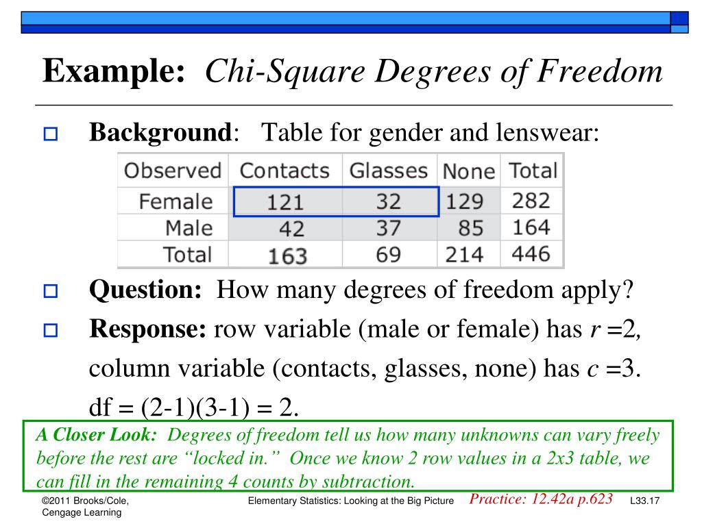
Conceptually, the degrees of freedom for a contingency table are the number of cell counts that are free to vary after the row and column totals are fixed.

Imagine a simple 2x2 table. If you know the row totals and the column totals, you only need to know the value of one cell. Once that single cell is filled in, all other cell values are automatically determined to make the totals add up correctly. Therefore, a 2x2 table has only 1 degree of freedom.

This logic extends to larger tables, leading to a simple formula:

The following video provides an excellent visual and intuitive explanation of this concept.

The degrees of freedom determine the specific chi-square probability distribution we use to evaluate our test statistic. Different degrees of freedom result in differently shaped distributions.

Conclusion

In this lesson, we deconstructed the Pearson chi-square test, moving from the logic of hypothesis testing to the mechanics of calculating a test statistic. You now have the tools to quantify the evidence against a claim of independence.

Key Takeaways:

• The Pearson ${\chi }^2$ statistic is a measure of the total discrepancy between the observed counts ($O$) in your sample and the expected counts ($E$) that would occur if the null hypothesis of independence were true.
• Expected counts are calculated for each cell using the formula: $E=(\text{row total}\times \text{column total})/\text{grand total}$.
• The chi-square formula, ${\chi }^2=\sum \frac{(O-E{)}^2}{E}$, sums the standardized squared deviations across all cells to produce a single test statistic.
• The degrees of freedom ($df$) determine the specific chi-square distribution used for comparison and are calculated as $df=(r-1)(c-1)$.

Preview of the Next Lesson:

We now know how to calculate the ${\chi }^2$ statistic and its degrees of freedom. But what are the rules for using this test? In the next lesson, we will discuss the critical assumptions of the chi-square test, particularly regarding sample size and expected counts. You'll learn how to check these assumptions and what to do when they are violated, which will lead us directly to an important alternative: Fisher's exact test.