Understanding and Applying Ordinal Logistic Regression

1. When is Ordinal Logistic Regression Appropriate?

Ordinal logistic regression is the right choice when your dependent variable has three or more categories that follow a natural, meaningful order. Using a model that acknowledges this order is generally better than using multinomial regression for two main reasons:

1. More Statistical Power: By incorporating the ordering information, the model can detect relationships between predictors and the outcome more effectively.
2. Parsimony: As we will see, the model is simpler and has fewer parameters to estimate than a comparable multinomial model, which makes interpretation easier.

The table below provides a clear distinction between the logistic regression models we've covered so far.

To begin, let's watch a short video that introduces the concept of ordinal response variables and why using a specialized model is advantageous.

2. The Core Mechanism: Cumulative Probabilities and Logits

So, how does the model use the ordering information? Instead of modeling the probability of being in a specific category (like multinomial regression does), ordinal regression models the probability of being in a category at or below a certain level. This is called the cumulative probability.

Let's say our outcome $Y$ has $J$ ordered categories: $1,2,\dots ,J$. The model works with the following probabilities:

• $P(Y\le 1)$
• $P(Y\le 2)$
• ...
• $P(Y\le J-1)$

Notice that $P(Y\le J)$ is always 1, so we only need to model $J-1$ cumulative probabilities.

By doing this, we've reframed the multi-category problem into a series of $J-1$ binary comparisons:

• Is the outcome in category 1, or is it higher? (Category 1 vs. {2, 3, ..., J})
• Is the outcome in category 1 or 2, or is it higher? ({1, 2} vs. {3, ..., J})
• ... and so on.

The model then takes the logit of each of these cumulative probabilities. This is called the cumulative logit.

The next segment of the video provides a clear numerical example of how these cumulative probabilities and their corresponding logits are calculated.

3. The Proportional Odds (Cumulative Logit) Model

Now that we understand cumulative logits, we can define the model itself. The proportional odds model is the most common type of ordinal logistic regression. It models each of the $J-1$ cumulative logits as a function of the predictor variables.

For a single predictor $x$, the model is defined by a set of equations:

Let's break this down:

• ${\alpha }_j$ (The Intercepts or Thresholds): Notice that the intercept $\alpha$ has a subscript $j$. This means there is a different intercept for each cumulative logit. These intercepts are often called thresholds or cut-points, as they define the boundaries between the cumulative probabilities.
• $\beta$ (The Slope): Crucially, the coefficient $\beta$ for the predictor $x$ is the same across all $J-1$ equations. This is the proportional odds assumption. It implies that the effect of the predictor $x$ on the odds of being at or below category $j$ is the same, no matter which category $j$ you choose as the cut-point.

The video you've been watching explains this model structure very well.

Visualizing the Proportional Odds Assumption

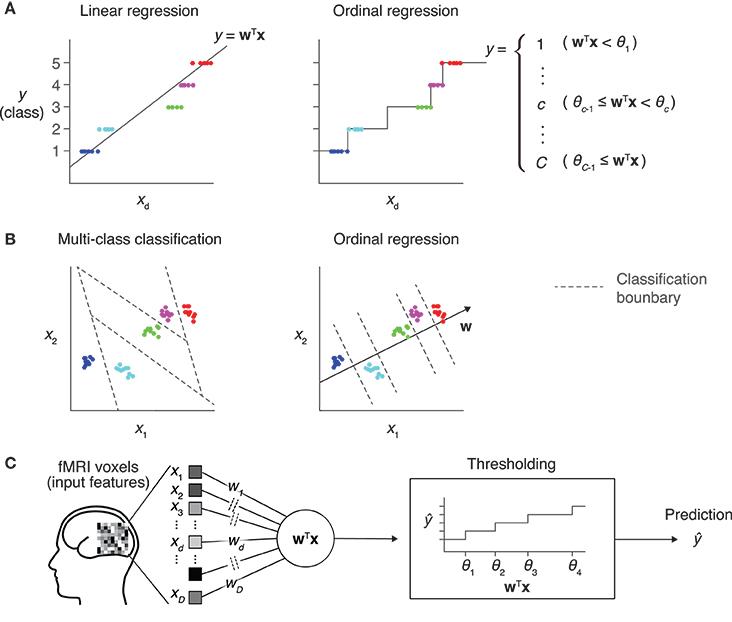
The assumption of a single $\beta$ means the model estimates a set of parallel lines or planes—one for each cumulative logit. The distance between the lines is determined by the different intercepts (${\alpha }_j$).

The image below provides an excellent visual intuition for this. Panel B contrasts a multi-class model (like multinomial regression), which can have boundaries in any direction, with an ordinal model, where the boundaries are parallel.

Why is it called "Proportional Odds"?

To understand the name, let's rearrange the model equation to look at the cumulative odds:

If we increase $x$ by one unit, the new odds will be $e^{{\alpha }_j-\beta (x+1)}$. The ratio of the new odds to the old odds is:

This odds ratio, $e^{-\beta }$, is constant for any value of $x$ and, most importantly, for any cut-point $j$. The effect of the predictor is proportional across all the odds equations, hence the name "proportional odds."

The following reading provides a detailed explanation of the model, including its interpretation and a very helpful analogy to an underlying continuous variable.

Conclusion

In this lesson, we introduced ordinal logistic regression as a specialized tool for modeling dependent variables with ordered categories. You learned why this approach is preferable to multinomial regression and how its most common form, the proportional odds model, works.

Key Takeaways:

• When to use it: Ordinal logistic regression is appropriate for response variables with three or more categories that have a natural order.
• Core concept: The model works with cumulative probabilities ($P(Y\le j)$) and their corresponding cumulative logits.
• Model Structure: The proportional odds (or cumulative logit) model has separate intercepts (${\alpha }_j$) for each cumulative split but assumes a common set of slope coefficients ($\beta$) for the predictors.
• Proportional Odds Assumption: This core assumption means that the effect of a predictor on the odds of being in a lower versus a higher category is the same across all possible cut-points of the outcome. This leads to a simpler, more parsimonious model.

Preview of the Next Lesson:

The proportional odds assumption is what gives the model its power and simplicity, but it's a strong assumption that may not always hold true. What if the effect of a predictor is different for distinguishing "low" from "medium/high" than it is for distinguishing "low/medium" from "high"? In our next lesson, we will learn how to formally test the proportional odds assumption and discuss what to do if it is violated.