Interpreting Multinomial Logistic Regression Coefficients

1. The Core Idea: One Model, Multiple Equations

As a quick refresher, remember that a multinomial model doesn't produce just one set of coefficients. If your outcome has K categories, you'll get K-1 sets of coefficients. Each set belongs to an equation that models the log-odds of being in one specific category versus the reference category.

Let's watch a short video that uses a concrete example to show how these equations are structured and how to interpret the resulting coefficients.

As the video demonstrated, the interpretation always involves three parts: the predictor, the outcome category, and the reference category. For instance, "the odds of being unemployed versus in employment are 42% lower for women than for men."

2. A Practical Example: Choosing a High School Program

Let's ground our learning in a new, slightly more complex example. We'll use a dataset containing information on 200 students. Our goal is to model their choice of academic program.

• Dependent Variable (Y): prog - Program type, with three categories:
  1. general
  2. academic
  3. vocational
• Predictor Variables (X):
  • ses - Social economic status (a categorical variable: "low", "middle", "high")
  • math - Standardized math score (a continuous variable)
  • science - Standardized science score (a continuous variable)

Since the program choice is a nominal variable with three categories, multinomial logistic regression is the perfect tool.

3. Fitting and Interpreting the Model

For this analysis, we will set 'academic' as the reference category. This is a common choice as it is the largest group in the dataset. Therefore, our model will produce two sets of coefficients:

1. One for comparing general vs. academic.
2. One for comparing vocational vs. academic.

The resource below walks through the process of fitting this model in R and provides the output tables we will analyze.

Deconstructing the Output

After running the model, the software provides a table of coefficients. It typically looks something like this, with one row for each non-reference category comparison:

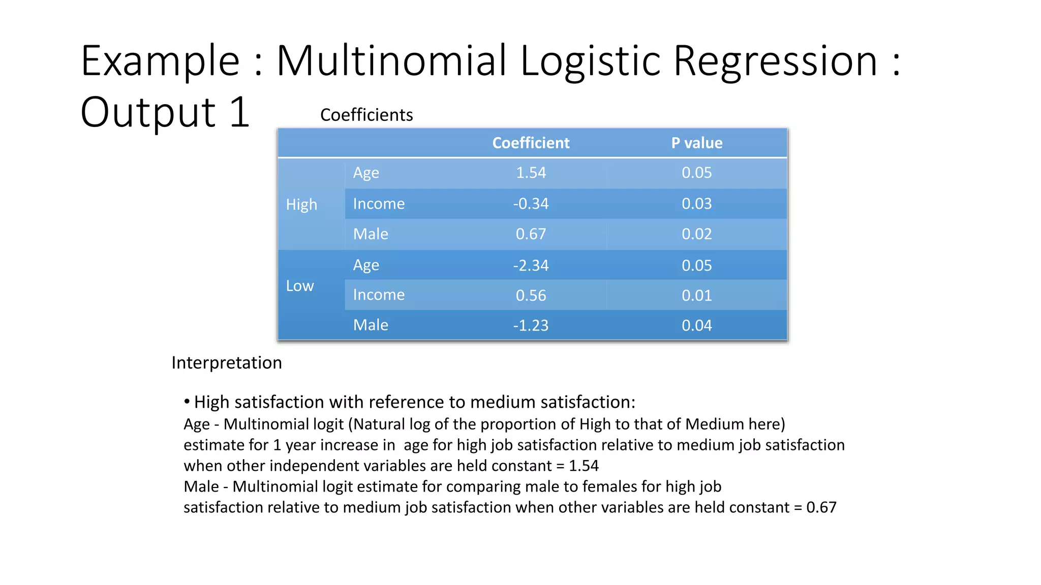
Let's use the output from our high school program example in the reading to interpret the coefficients.

A. Interpreting Coefficients as Log-Odds

The raw coefficients are on the log-odds scale.

• Coefficient for ses="low" (vs. high) on general: The reading notes the coefficient is -1.125.

  • Interpretation: For a student with low SES compared to a student with high SES, the log-odds of being in the general program versus the academic program decrease by 1.125. This suggests low-SES students are less likely to choose the general program over the academic one, compared to high-SES students.

• Coefficient for math on vocational: The coefficient is -0.504.

  • Interpretation: For each one-point increase in a student's math score, the log-odds of being in the vocational program versus the academic program decrease by 0.504. Higher math scores make it less likely a student will choose a vocational path over an academic one.

B. Interpreting Coefficients as Odds Ratios

To make the interpretation more intuitive, we exponentiate the coefficients to get odds ratios.
Let's use the odds ratios provided in the R lab reading (exp(coef(multi_mo))).

• Odds Ratio for ses="middle" (vs. high) on vocational: The coefficient is 0.840. The odds ratio is $e^{0.840}\approx 2.31$.

  • Interpretation: The odds of choosing the vocational program over the academic program are 2.31 times higher for a student from a middle-SES background compared to a student from a high-SES background.

• Odds Ratio for math on general: The coefficient is -0.185. The odds ratio is $e^{-0.185}\approx 0.83$.

  • Interpretation: For each one-point increase in math score, the odds of choosing the general program over the academic program are multiplied by 0.83 (i.e., they decrease by about 17%).

Notice every interpretation specifies the comparison category (general vs academic) and the reference group for the predictor if it's categorical (middle SES vs high SES).

4. From Coefficients to Probabilities

Interpreting individual coefficients is crucial, but it can be hard to see the big picture, especially with many predictors. A more holistic way to understand the model is to use it to predict the probability of each outcome for specific profiles of interest.

In the last lesson, you saw the softmax formula that turns log-odds into probabilities. Let's see it in action.

This process allows us to make powerful summary statements. For our high school example, we could calculate the predicted probabilities for two hypothetical students:

• Student A: Low SES, 40 math score, 40 science score
• Student B: High SES, 70 math score, 70 science score

We would likely find that Student A has a higher probability of being in the vocational or general program, while Student B has a very high probability of being in the academic program. This is often more insightful than interpreting each coefficient in isolation.

5. Visualizing the Model's Predictions

When you have two continuous predictors, you can create a plot of the decision boundaries. This plot shows how the model divides the predictor space into regions where each outcome category is the most likely.

This visualization provides an excellent intuitive feel for what the model has learned. The coefficients we interpret define the precise location and slope of these boundaries. The model essentially learns a set of rules to partition the data, and the decision boundaries are the visual representation of those rules.

Conclusion

In this lesson, we bridged the gap from theory to practice, focusing on how to fit a multinomial logistic regression model and interpret its output.

Key Takeaways:

• A multinomial model with a K-category outcome produces K-1 sets of coefficients, each comparing an outcome category to a chosen reference category.
• Coefficients can be interpreted as either log-odds or, more intuitively, as odds ratios. The interpretation must always state the two outcome categories being compared (e.g., vocational vs. academic).
• While coefficient-level interpretation is detailed, a more holistic understanding comes from calculating and comparing predicted probabilities for different predictor profiles.
• Decision boundaries provide a powerful visual representation of how the model classifies observations based on their predictor values.

Preview of the Next Lesson:

We've now covered models for binary outcomes and nominal outcomes. But what if the categories have a natural order (e.g., "low," "medium," "high")? Standard multinomial regression ignores this ordering. In our next lesson, we will explore ordinal logistic regression, a model specifically designed to leverage the information contained in ordered categorical variables.