Interpreting Ordinal Logistic Regression Coefficients

1. The Challenge and the Strategy for Interpretation

Interpreting ordinal regression coefficients can be confusing at first. This is because of the way most statistical software (like R's polr package and Stata's ologit command) parameterizes the model with a negative sign before the $\beta$ coefficient.

This can lead to interpretations involving double negatives, which are hard to grasp. For instance, a positive coefficient means an increase in the predictor is associated with a decrease in the log-odds of being in a lower outcome category.

Fortunately, there is a much more straightforward way to think about and state this relationship. By slightly reframing the odds we are looking at, we can arrive at an interpretation that is both correct and easy to understand.

Let's dive into a resource that explains this strategy perfectly.

To summarize the key insight from that reading:

If a predictor $x$ has a coefficient $\beta$, the odds ratio is $e^{\beta }$. The most intuitive way to interpret this is:
For a one-unit increase in $x$, the odds of the outcome being in a higher category (versus a lower category) are multiplied by a factor of $e^{\beta }$.

• If $\beta >0$, then $e^{\beta }>1$, and an increase in $x$ is associated with higher odds of being in a higher outcome category.
• If $\beta <0$, then $e^{\beta }<1$, and an increase in $x$ is associated with lower odds of being in a higher outcome category.

This single odds ratio applies across all $J-1$ possible splits of the outcome variable, due to the proportional odds assumption.

2. A Worked Example: Interpreting Model Output

Let's solidify this with the example from the reading and a video walkthrough. The model examines how parental education (pared, where 1 = at least one parent has a degree) predicts a student's likelihood of applying to college (apply, with categories: "unlikely", "somewhat likely", "very likely").

The video below shows the output from Stata and demonstrates how to interpret the coefficient for pared.

Based on the video, the interpretation is:

For students who have at least one parent with a degree, the odds of being in a higher application likelihood category (e.g., 'very likely' vs. 'somewhat or unlikely', OR 'very or somewhat likely' vs. 'unlikely') are 3.09 times the odds for students whose parents do not have a degree.

3. What About the Intercepts?

The model output also includes several intercepts, sometimes called thresholds or cut-points. While our primary focus is usually on the predictor coefficients ($\beta$), it's important to know what these represent.

In short, the intercepts (${\alpha }_j$) are the estimated log-odds of being in category $j$ or below when all predictor variables are held at their baseline value (usually zero). They establish the baseline boundaries between the outcome categories.

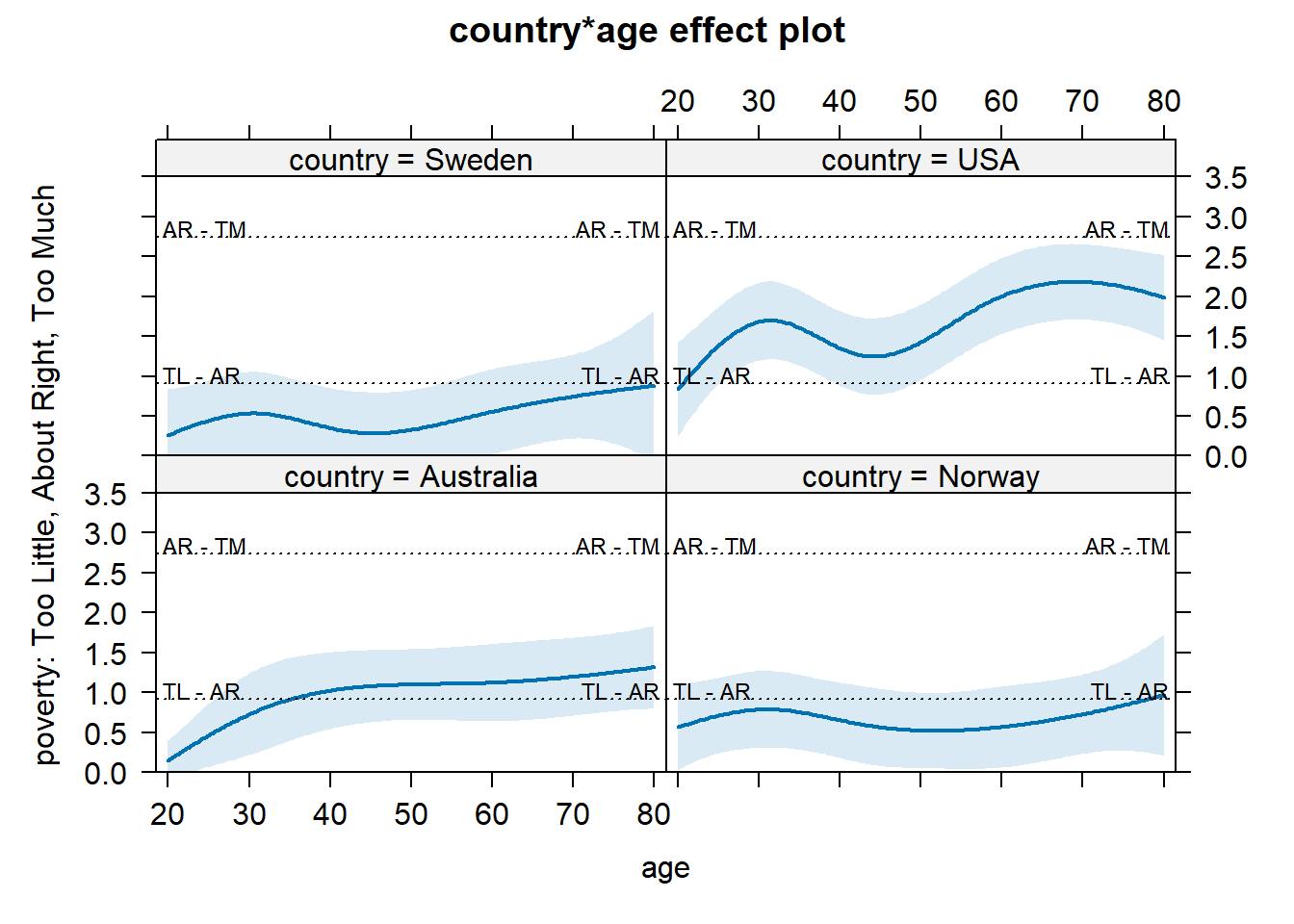
The intercepts define the locations of the parallel lines or planes that separate the outcome categories. The image below visualizes these thresholds (the horizontal dotted lines) for a model predicting perceptions of poverty based on age in different countries.

4. For Functional Understanding: From Odds Ratios to Probabilities

As you've emphasized, functional understanding is key. While odds ratios are the correct way to interpret the coefficients directly, they can be abstract. For communicating results to a broader audience, converting the model's output into predicted probabilities is often far more effective.

Using the full model—both the intercepts (${\alpha }_j$) and the slope ($\beta$)—we can calculate the predicted probability of an individual falling into each specific outcome category, given their values on the predictor variables.

The process involves two steps:

1. Calculate the cumulative probabilities $P(Y\le j)$ for each cut-point.
2. Use subtraction to find the probability for each individual category: $P(Y=j)=P(Y\le j)-P(Y\le j-1)$.

The next segment of the video demonstrates this calculation and shows how to present the results in a simple, powerful table.

Presenting a table showing that students with educated parents have a 21% chance of being "very likely" to apply, compared to only 8% for students without educated parents, is a much more direct way to communicate the practical significance of the predictor.

Conclusion

In this lesson, we focused on the practical interpretation of coefficients from an ordinal logistic regression model. You learned a clear strategy to navigate the potential confusion caused by model parameterization and how to communicate your findings effectively.

Key Takeaways:

• Main Interpretation Strategy: To interpret a coefficient $\beta$, exponentiate it to get the odds ratio $e^{\beta }$. This value represents the multiplicative change in the odds of being in a higher outcome category for a one-unit increase in the predictor.
• Positive vs. Negative Coefficients: A positive $\beta$ ($e^{\beta }>1$) means the predictor is associated with higher levels of the outcome. A negative $\beta$ ($e^{\beta }<1$) means the predictor is associated with lower levels of the outcome.
• Intercepts are Thresholds: The intercepts (${\alpha }_j$) represent the baseline cut-points between the ordered categories on the log-odds scale.
• Communicate with Probabilities: While odds ratios are the direct interpretation, calculating and presenting predicted probabilities for each outcome category is often the most intuitive way to convey the model's practical implications.

Preview of the Next Lesson:

The entire interpretation we learned today hinges on the proportional odds assumption—the idea that $\beta$ is the same across all category splits. But what if this assumption is wrong? In our next lesson, we will learn how to state and test the proportional odds assumption and discuss what to do if the test reveals a problem.