Creating Delta Tables with CTAS

1. From Transformation to Table: The CTAS Pattern

In data engineering, a common workflow is to read raw data, apply a series of transformations (like cleaning, filtering, or joining), and then save the cleaned-up data into a new table. CTAS is designed for exactly this purpose. It combines two operations into one:

1. CREATE TABLE: It defines a new table.
2. AS SELECT ...: It populates that new table with the data returned by your SELECT query.

The schema of the new table is automatically inferred from the columns in your SELECT statement. In Databricks, the default table format is Delta Lake, so when you use CTAS, you are creating a reliable, high-performance Delta table.

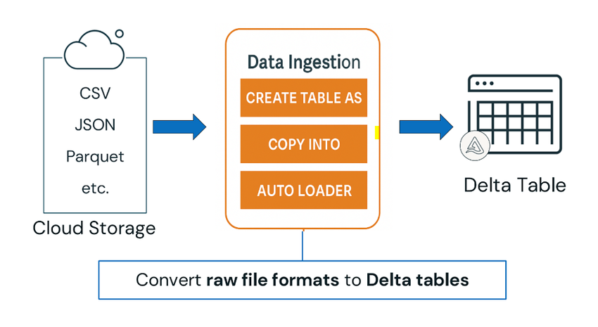
This diagram shows where CTAS fits into the broader data ingestion landscape. It's one of the primary methods for converting data from various sources into the Delta format.

2. The Basic Syntax

The simplest form of a CTAS statement is straightforward. You define the new table's name and then provide the query that will generate its data.

For a deeper dive into the syntax and a clear example, let's turn to a short reading.

As the article shows, the basic structure is:

CREATE TABLE new_table_name
AS
SELECT column1, some_transformation(column2)
FROM existing_table
WHERE condition;

This single command executes the SELECT query and creates new_table_name containing its results.

3. Hands-On Practice: Persisting a CTE Result

Let's connect this back to what we learned in the last lesson about CTEs. A common and powerful pattern is to use CTEs to define a complex, multi-stage transformation and then use CTAS to save the final result.

Instructions:
Open a Databricks SQL notebook and follow these steps.

Step 1: Create Sample Data
First, let's create a table with some sample sales data. This represents our raw source.

CREATE OR REPLACE TABLE raw_sales (
  order_id INT,
  product_category STRING,
  quantity INT,
  unit_price DECIMAL(10, 2),
  order_date DATE
);

INSERT INTO raw_sales VALUES
  (101, 'Electronics', 1, 1200.00, '2023-10-01'),
  (102, 'Books', 5, 15.50, '2023-10-01'),
  (103, 'Electronics', 2, 800.00, '2023-10-02'),
  (104, 'Home Goods', 10, 25.00, '2023-10-03'),
  (105, 'Books', 2, 22.00, '2023-10-03');

Step 2: Build and Persist the Transformation
Now, imagine our goal is to create an aggregated daily sales summary table specifically for the 'Electronics' category. We'll first define the logic with a CTE and then wrap it in a CREATE OR REPLACE TABLE ... AS statement.

Using CREATE OR REPLACE instead of just CREATE makes our code idempotent, meaning we can run it multiple times without causing an error on subsequent runs. This is a best practice for production data pipelines.

Execute the following query:

CREATE OR REPLACE TABLE electronics_daily_summary AS
WITH
  electronics_sales AS (
    SELECT
      order_date,
      quantity,
      unit_price
    FROM
      raw_sales
    WHERE
      product_category = 'Electronics'
  )
SELECT
  order_date,
  SUM(quantity * unit_price) AS total_revenue,
  COUNT(order_date) AS number_of_orders
FROM
  electronics_sales
GROUP BY
  order_date
ORDER BY
  order_date;

Step 3: Verify the Result
Your transformation is now complete, and the results are saved. You can query the new table to see the output:

SELECT * FROM electronics_daily_summary;

You should see a new table containing the aggregated daily revenue and order count for electronics. You've successfully used a CTE to define a transformation and CTAS to materialize it.

4. CTAS in a Real-World Scenario

The example above used an existing table as a source. In many real-world ELT scenarios, you will create tables directly from raw files (like CSVs or JSON) stored in cloud storage.

The following article walks through a great practical example: building a product dimension table for a retail business by reading data directly from CSV files.

This article showcases how a single, elegant CTAS statement can handle file ingestion, schema definition, data type casting, and table creation all in one step.

5. Important Variations: Managed vs. External Tables

So far, we've created managed tables, where Databricks controls both the metadata and the underlying data files. If you drop a managed table, the data is deleted.

Sometimes, you need to create an external table, where Databricks manages the metadata, but the data files reside in an external location you specify (e.g., an S3 bucket or ADLS container). If you drop an external table, the underlying data files remain untouched.

You can use CTAS to create an external table by simply adding a LOCATION clause. The following video demonstrates this and other useful CTAS patterns.

6. CTAS vs. CLONE

When working with Delta Lake, you might also hear about the CLONE command. It's important to understand the difference.

• CTAS (CREATE TABLE AS SELECT): Creates a new table based on the result of a query. This is for transformation. The new table has its own, separate history.
• CLONE: Creates a copy of an existing Delta table at a specific version.
  • DEEP CLONE copies both the data and the metadata. This is for creating an independent, identical replica.
  • SHALLOW CLONE copies only the metadata and points to the original data files. This is for creating a lightweight copy for quick experiments without duplicating data.

Use CTAS when you are changing the data's structure or content. Use CLONE when you need an exact replica for backups, testing, or development.

This short video segment clarifies the distinction.

Conclusion

You now have a powerful tool in your data engineering arsenal. The CREATE TABLE AS SELECT statement bridges the gap between defining a transformation and persisting its result, forming the backbone of many ELT pipelines in Databricks.

Key Takeaways

• CTAS is a single command that creates and populates a new Delta table from the results of a SELECT query.
• It's the standard method for materializing transformations into physical tables.
• Using CREATE OR REPLACE TABLE ... AS SELECT is a best practice for creating idempotent pipelines that can be re-run safely.
• You can create an external table by adding a LOCATION 'path/to/data' clause to your CTAS statement.
• Use CTAS for transformation and CLONE for exact replication of Delta tables.

Next Steps

In this lesson and the last, you've focused on the structure of transformation queries and how to save their results. In the next lesson, we will zoom in on the SELECT clause itself and begin exploring the rich library of built-in Spark SQL functions, starting with functions for string manipulation.