Hello! Let's dive into the second lesson of our module on Transforming Data with Spark SQL.
In the previous lesson, we explored how to use temporary views to modularize transformation logic across an entire Spark session. This is great for breaking a large pipeline into reusable, named components. But what if you only need to structure the logic within a single, complex query? Writing nested subqueries can quickly become confusing and difficult to maintain.
This lesson introduces a powerful solution: Common Table Expressions (CTEs). You will learn how to use the WITH clause to define temporary, named result sets that exist only for the duration of a single query. Mastering CTEs is essential for writing clean, readable, and maintainable multi-stage ELT queries in Spark SQL.
1. From Nested Subqueries to Readable Logic
As you know from your data analytics experience, it's common to need to perform a calculation on the result of another calculation. Often, this leads to writing queries inside other queries, known as subqueries. When these are nested, they can be hard to read because you have to mentally unpack them from the inside out.
A Common Table Expression (CTE) provides a way to solve this. Think of it as a temporary, named result set that you define at the beginning of your query using a WITH clause. This allows you to break down a complex query into a series of logical, sequential steps, dramatically improving readability.
To see a direct comparison, the following video walks through a problem, first solving it with confusing nested subqueries and then refactoring the exact same logic into a clean, step-by-step query using CTEs.
SQL WITH Clause | How to write SQL Queries using WITH Clause | SQL CTE (Common Table Expression)
This video from techTFQ provides an excellent demonstration of why CTEs are so useful. Pay close attention to how the presenter transforms a hard-to-read query into a much cleaner version.
Watch the segment from 06:25 to 18:30. You will see the presenter: Define a multi-step problem: find stores with sales greater than the average sales across all stores. First, solve it using nested subqueries, highlighting the readability issues and repeated logic. Then, rewrite the solution using CTEs to define each logical step (total_sales, average_sales) separately before combining them in the final SELECT statement.
As the video clearly shows, the CTE version is structured like a recipe: first, you prepare the total_sales, then you use that to prepare the average_sales, and finally, you use both to get your result. This sequential flow is much easier to understand, debug, and maintain.
2. The Anatomy of a CTE Query
The fundamental syntax for a CTE is the WITH clause, which precedes your main SELECT statement.
A single CTE looks like this:
WITH my_cte_name AS (
  -- This is the query that defines the CTE
  SELECT column1, column2 FROM some_table WHERE condition
)
-- This is the main query that uses the CTE
SELECT * FROM my_cte_name;
The real power of CTEs comes from chaining them together. You can define multiple CTEs, and a later CTE can refer to an earlier one. This is how you build sequential transformation pipelines.
WITH
  cte_1 AS (
    SELECT ... FROM source_table  -- Step 1: Initial filtering/transformation
  ),
  cte_2 AS (
    SELECT ... FROM cte_1         -- Step 2: Build on the result of Step 1
  )
SELECT ... FROM cte_2;           -- Step 3: Final query using the last CTE
This structure creates a clear, top-to-bottom data flow within your query.
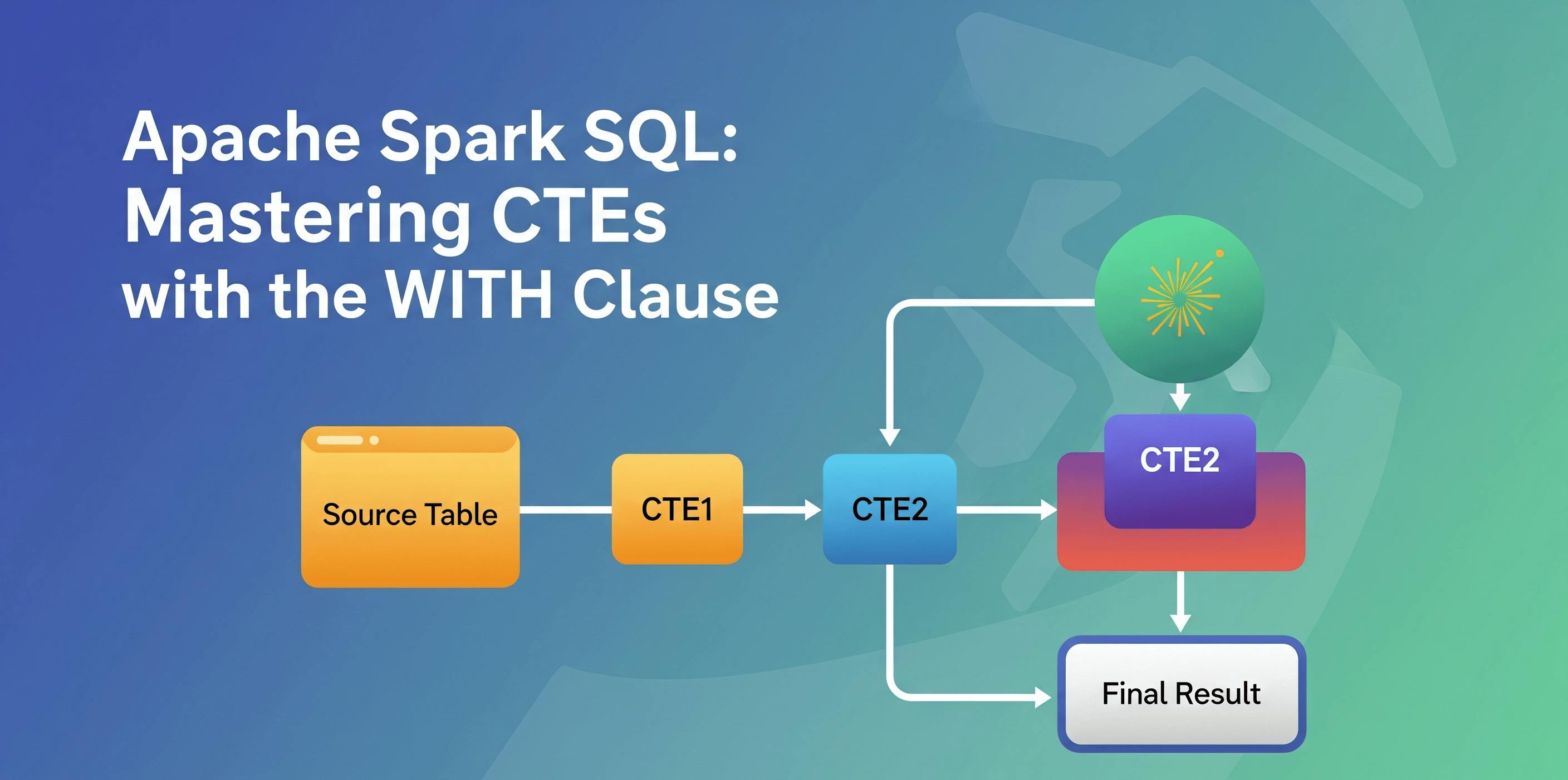
Now, let's look at a text resource that shows this chaining in action and how to execute it in a Databricks notebook.
25: PySpark SQL With Common Table Expression (i.e. CTE)
The article "PySpark SQL With Common Table Expression" provides a concise, practical example of chaining CTEs to find top-rated marketing campaigns.
Please read the following two sections under the heading "Common Table Expression (i.e. CTE) approach": "Step 5: Directly as SQL": This shows the SQL code for a two-step CTE. Notice how the first CTE, avg_rating, calculates an average, and the second CTE, rating_ranked, uses avg_rating to perform a window function. "Step 6: Spark SQL with Python notebook": This shows how you can wrap the exact same multi-line SQL query into a string in PySpark and execute it with spark.sql(). This is a common pattern in Databricks.
3. Hands-On Practice: Staged Event Reconstruction
Let's apply this to a scenario that might be familiar from your physics background: reconstructing particle events from detector data. We will perform a multi-stage analysis where each stage is a CTE.
Imagine we have a table of raw signals from a detector. Our goal is to find the average reconstructed energy per detector region, but only for high-quality, multi-particle events.
Instructions:
Open a new Databricks SQL notebook and execute the following queries step-by-step.
Step 1: Set Up the Raw Data
First, run this query to create our source table with raw detector signals.
CREATE OR REPLACE TABLE raw_detector_signals (
  event_id INT,
  region_id STRING,
  signal_strength DOUBLE,
  signal_to_noise_ratio DOUBLE,
  particle_count INT
);

INSERT INTO raw_detector_signals VALUES
  (1, 'A', 150.5, 3.1, 1),
  (2, 'B', 875.2, 12.5, 3),
  (3, 'A', 950.1, 15.3, 4),
  (4, 'C', 220.0, 4.0, 1),
  (5, 'B', 450.7, 7.8, 2),
  (6, 'A', 1230.9, 25.1, 5),
  (7, 'C', 15.2, 1.5, 1);
Step 2: Build the Multi-Stage CTE Query
Now, we'll build our analysis query. We will define two CTEs to perform the filtering and transformation in sequence.
Copy and paste the entire query below into a new cell and then we'll break down what it does.
WITH
  -- Step 1: Filter for high-quality, multi-particle events
  high_quality_events AS (
    SELECT
      event_id,
      region_id,
      signal_strength,
      particle_count
    FROM raw_detector_signals
    WHERE
      signal_to_noise_ratio > 10.0 AND particle_count > 1
  ),

  -- Step 2: Reconstruct energy from the high-quality events
  reconstructed_energy AS (
    SELECT
      region_id,
      -- A simple physics-inspired "reconstruction" formula
      (signal_strength * 0.8) / particle_count AS reconstructed_energy_tev
    FROM high_quality_events
  )

-- Final Step: Aggregate the results
SELECT
  region_id,
  COUNT(*) AS num_high_quality_events,
  AVG(reconstructed_energy_tev) AS avg_reconstructed_energy_tev
FROM reconstructed_energy
GROUP BY region_id
ORDER BY region_id;
Let's analyze the flow:
- The first CTE,
high_quality_events, acts as our initial filter. It selects only the rows that meet our quality criteria from the source table. - The second CTE,
reconstructed_energy, reads exclusively fromhigh_quality_events. It applies a formula to calculate a new value,reconstructed_energy_tev. This is our transformation step. - The final
SELECTstatement reads fromreconstructed_energyto perform the final aggregation and produce our desired result.
When you run the query, you should see the final analysis, showing the number of qualifying events and the average reconstructed energy for regions 'A' and 'B'. This demonstrates a clear, sequential ELT flow within a single query.
4. CTEs vs. Temporary Views
It's important to be clear on when to use a CTE and when to use a temporary view (from the last lesson).
| Feature | Common Table Expression (CTE) | Temporary View |
|---|---|---|
| Scope | Query-scoped: Exists only for the duration of a single query. | Session-scoped: Exists for the entire Spark session. |
| Definition | WITH clause |
CREATE TEMPORARY VIEW |
| Primary Use | Breaking down a single complex query into logical, readable steps. | Modularizing logic to be reused across multiple queries in a notebook or job. |

In short:
- Use a CTE to organize the steps inside one query.
- Use a Temporary View to organize results you want to use across multiple, separate queries in your notebook.
Conclusion
You've now learned how to use Common Table Expressions to structure complex SQL logic. This skill is invaluable for any data engineer building transformation pipelines, as it makes your code significantly more readable and easier to debug than traditional nested subqueries.
Key Takeaways
- CTEs are defined using the
WITHclause and create temporary, named result sets that exist only for the scope of a single query. - They are used to break down complex logic into a series of sequential, readable steps.
- CTEs can be chained, allowing one CTE to build upon the results of a previous one, which is perfect for multi-stage transformations.
- CTEs are query-scoped, whereas temporary views are session-scoped.
Next Steps
Now that you can write sophisticated queries to transform data using both temporary views and CTEs, the next logical step is to persist the results of these transformations. In our next lesson, we will cover the CREATE TABLE AS SELECT (CTAS) statement, a powerful command that lets you create a new Delta table directly from the output of a SELECT query.