Transforming DataFrames: Adding, Modifying, and Ordering Columns

1. Adding and Modifying Columns with withColumn()

The primary tool for adding or updating a column in a PySpark DataFrame is the withColumn() method. Its signature is withColumn(colName, col), where colName is the name of the column you want to create or replace, and col is a Column expression that defines its values.

Let's start with a foundational reading that explains this transformation.

As the article explains, you can use withColumn() for two main purposes:

1. Add a new column: If the colName you provide doesn't exist, a new column is added to the DataFrame.
2. Overwrite an existing column: If the colName already exists, its values are replaced by the new calculation. This is useful for tasks like casting data types or standardizing values.

Here is a common syntax pattern using functions from pyspark.sql.functions:

from pyspark.sql.functions import col, lit, concat




# Example: Adding a new column with a literal (constant) value
df_with_new_col = df.withColumn("source_system", lit("SystemA"))




# Example: Overwriting an existing column by calculating a new value
# Let's say we have a 'price' column and want to add tax
df_with_tax = df.withColumn("price", col("price") * 1.1)

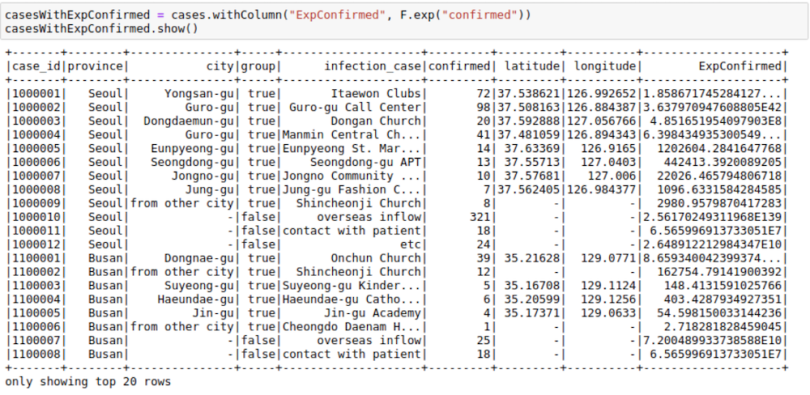
The image below shows another practical example of withColumn in action.

A Note on Performance

While chaining withColumn() calls is a very common pattern, it's important to be aware of the performance implications, especially as you advance in data engineering. Since DataFrames are immutable, each transformation theoretically creates a new DataFrame. When complex operations are involved, this can lead to performance issues.

The following video discusses an important performance optimization technique: using a single select() statement instead of multiple withColumn() calls when adding several columns.

For now, using withColumn() is perfectly fine, but keeping this optimization in mind will serve you well as you prepare for the certification exam and real-world projects.

2. Sorting DataFrames with orderBy() and sort()

By default, the rows in a Spark DataFrame are not guaranteed to be in any particular order because the data is distributed across multiple partitions in the cluster. To enforce an order, you must explicitly use a sorting transformation. PySpark provides two equivalent methods for this: orderBy() and sort().

This video provides a complete guide to using these functions.

To summarize the key points from the video:

• Single-column sort:

  from pyspark.sql.functions import col, desc, asc
  
  
  
  
  # Sort by 'salary' in ascending order (default)
  df.orderBy("salary")
  
  
  
  # or explicitly
  df.orderBy(col("salary").asc())
  
  
  
  
  # Sort by 'salary' in descending order
  df.orderBy(col("salary").desc())
  

• Multi-column sort:

  
  
  
  # Sort by department (ascending), then by salary (descending)
  df.orderBy(col("department").asc(), col("salary").desc())
  

The following image provides another clear visual of single and multi-column sorting.

Like the withColumn performance tip, it's worth noting that sorting is one of the more computationally expensive operations in Spark. It often requires a "shuffle," where data is moved between worker nodes across the network. Always be intentional when you sort large datasets.

3. Hands-On Exercise

Let's apply these new transformations to the baby names dataset. Run the setup code from our last lesson in a Databricks notebook to load the data.

# Step 1: Set up paths (replace with your catalog/schema/volume)
catalog = "your_catalog_name"
schema = "your_schema_name"
volume = "your_volume_name"
path_volume = f"/Volumes/{catalog}/{schema}/{volume}"
file_name = "baby_names.csv"




# Step 2: Load the data into a DataFrame
df = spark.read.csv(f"dbfs:{path_volume}/{file_name}",
  header=True,
  inferSchema=True,
  sep=",")




# Step 3: Clean up column names for easier use
df_clean = df.withColumnRenamed("First Name", "FirstName") \
             .withColumnRenamed("County", "County") \
             .withColumnRenamed("Sex", "Gender") \
             .withColumnRenamed("Count", "Count") \
             .withColumnRenamed("Year", "Year")




# Let's see our starting point
df_clean.show(5)

Now, use withColumn() and orderBy() to complete the following tasks.

Your Tasks:

1. Create a New Column: Some people believe shorter names are easier to remember. Add a new integer column named NameLength to df_clean that contains the length of each FirstName.
2. Sort the Data: Create a new DataFrame that is sorted to show the longest names first. If two names have the same length, the one with the higher Count should appear first.
3. Display Results: Display the top 20 longest and most popular names, showing only the FirstName, NameLength, Count, and Year columns.

Solution Walkthrough:

Try to solve the exercise yourself before looking at the code below.

from pyspark.sql.functions import col, length, desc




# Task 1 Solution: Create a new column for name length
# We use the `length` function from pyspark.sql.functions
df_with_length = df_clean.withColumn("NameLength", length(col("FirstName")))

print("DataFrame with NameLength column added:")
df_with_length.show(5)





# Task 2 Solution: Sort by the new length column (desc) and then by Count (desc)
df_sorted = df_with_length.orderBy(col("NameLength").desc(), col("Count").desc())





# Task 3 Solution: Select the relevant columns and show the top 20
print("\nTop 20 longest and most popular names:")
df_sorted.select("FirstName", "NameLength", "Count", "Year").show(20)

Conclusion

Excellent work! You can now add new features to your data and present it in a sorted, meaningful order. These are essential transformations in any data pipeline.

Key Takeaways

• withColumn(colName, col) is the primary method for adding or overwriting columns.
• orderBy() and sort() are used to order a DataFrame's rows. They are aliases and can be used interchangeably.
• Sorting can be done on one or more columns, in either ascending (asc) or descending (desc) order.
• Both chaining withColumn and sorting with orderBy can be computationally expensive, so use them judiciously in production pipelines.

Next Steps

We've now covered selecting, filtering, transforming, and sorting data at the row and column level. The next logical step is to learn how to summarize data. In our next lesson, we will dive into groupBy() and aggregate functions, which allow you to compute summary statistics (like counts, sums, and averages) for groups of rows.