Closed-Loop Speed Control with MCPWM and PCNT

1. The Architecture of a Closed-Loop System

A closed-loop control system continuously measures a system's output (the Process Variable or PV) and compares it to a desired value (the Setpoint). The difference, or error, is fed into a controller, which calculates a corrective action to be applied by an actuator.

For our DC motor system, the components are:

• Setpoint: The target speed in RPM we want the motor to achieve.
• Sensor (PCNT): Measures the encoder pulses to determine the motor's current rotation.
• Controller (ESP32): Our C++ code that calculates the current speed, finds the error, and computes a new motor power level.
• Actuator (MCPWM + H-Bridge): Applies the calculated power level to the motor by adjusting the PWM duty cycle.
• Plant: The DC motor itself.

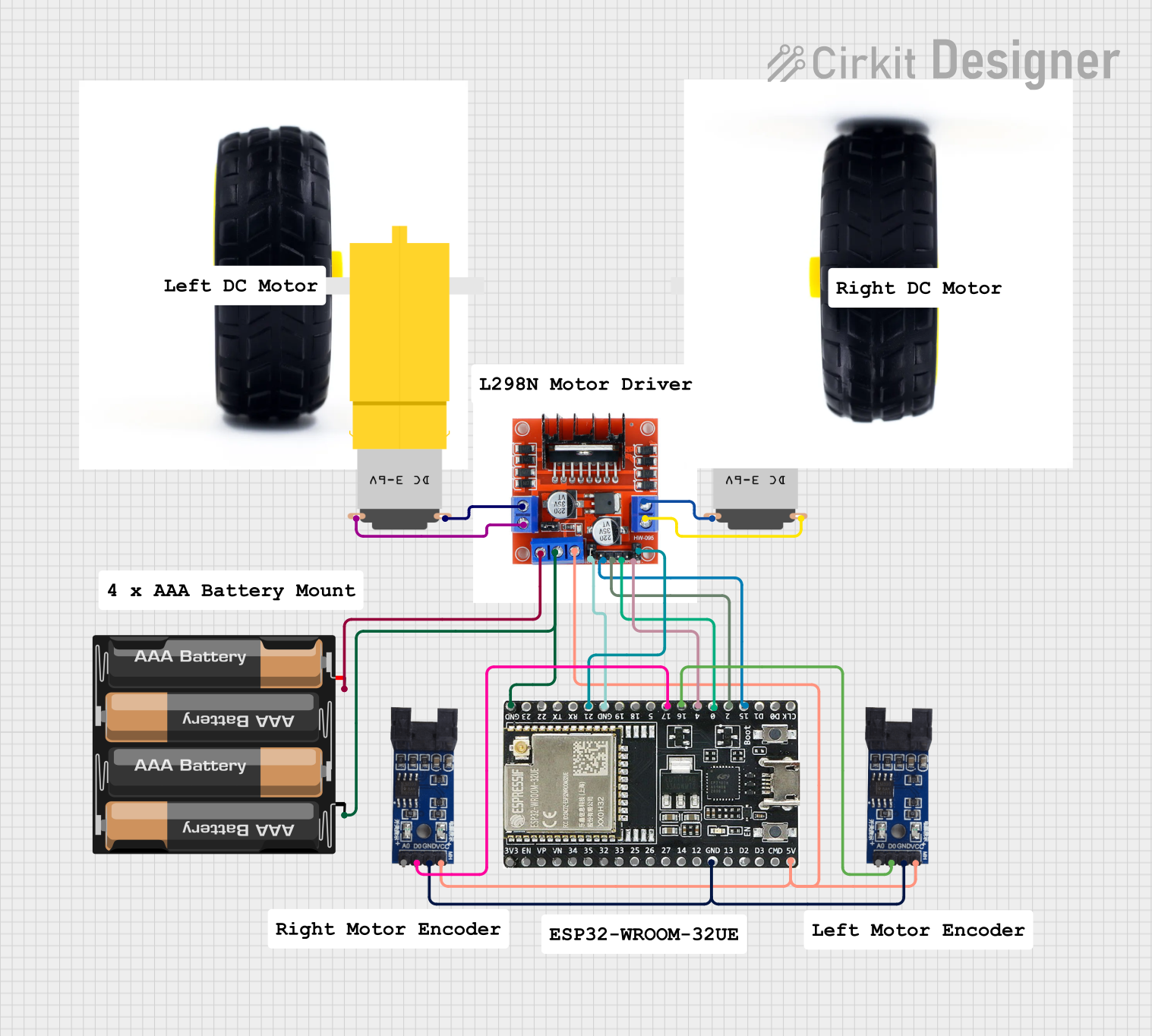
Our control loop will execute periodically:

1. Measure: Get the latest pulse count from the PCNT peripheral.
2. Calculate: Determine the actual motor speed (RPM) based on the change in pulse count over a fixed time interval.
3. Compare: Compute the error: error = target_speed - actual_speed.
4. Act: Calculate a new PWM duty cycle based on the error and update the MCPWM comparator.

2. From Pulses to Speed

The first step inside our control loop is to convert the raw pulse count from the PCNT into a meaningful speed measurement, like revolutions per minute (RPM).

To do this, we need to sample the pulse count at a regular interval. Let's say we read the counter every 100 milliseconds.

• count_at_t0: The pulse count from pcnt_unit_get_count() at the beginning of the interval.
• count_at_t1: The pulse count at the end of the interval (100 ms later).
• delta_counts = count_at_t1 - count_at_t0.
• delta_time_s: The sampling interval in seconds (0.1 s).

We also need to know the resolution of our encoder system, i.e., how many counts correspond to one full revolution. This depends on your encoder's native Pulses Per Revolution (PPR) and the decoding mode you used in the PCNT configuration. From the last lesson, if you are using 2x decoding with an encoder that has N pulses per revolution, then:

pulses_per_rev = 2 * N

The speed calculation is then:

$\text{Speed (RPM)}=\frac{\text{delta\_counts}}{\text{pulses\_per\_rev}}\times \frac{60}{\text{delta\_time\_s}}$

For example, if your 20-PPR encoder (using 2x decoding, so pulses_per_rev = 40) produces 30 counts in a 100 ms interval, the speed is:

$\text{Speed (RPM)}=\frac{30}{40}\times \frac{60}{0.1}=0.75\times 600=450\text{RPM}$

This calculation will be the core of our feedback measurement.

3. Implementing a Proportional (P) Controller

The simplest form of a feedback controller is a Proportional (P) controller. Its logic is straightforward: the corrective action is directly proportional to the size of the error.

$\text{Control Output}=K_p\times \text{error}$

Where:

• error = setpoint_speed - measured_speed.
• $K_p$ is the proportional gain, a tuning constant that determines how aggressively the controller reacts to error.

The Control Output must then be translated into a valid duty cycle for the MCPWM peripheral. A critical step is to combine this proportional correction with a baseline duty cycle and then constrain the result to the valid range (e.g., 0% to 100%).

A simple implementation might look like this:

// --- Inside your periodic control task ---

// 1. Calculate speed (as shown in the previous section)
float measured_speed = calculate_speed_from_encoder();

// 2. Calculate error
float error = target_speed - measured_speed;

// 3. Calculate proportional correction
float correction = Kp * error;

// 4. Calculate new duty cycle
// Start with the current duty and add the correction
float new_duty_cycle = current_duty_cycle + correction;

// 5. Clamp the duty cycle to a valid range (e.g., 0 to 100)
if (new_duty_cycle > 100.0f) {
    new_duty_cycle = 100.0f;
} else if (new_duty_cycle < 0.0f) {
    new_duty_cycle = 0.0f;
}

// 6. Update the hardware
// 'timer_period' is the value for 100% duty cycle
uint32_t mcpwm_compare_value = (uint32_t)(new_duty_cycle / 100.0f * timer_period);
ESP_ERROR_CHECK(mcpwm_comparator_set_compare_value(comparator, mcpwm_compare_value));

// Store the new duty cycle for the next iteration
current_duty_cycle = new_duty_cycle;

Tuning $K_p$:

• Low $K_p$: The controller reacts slowly. It may not be able to reach the setpoint, resulting in a large steady-state error.
• High $K_p$: The controller reacts aggressively. This can lead to overshoot (the speed exceeds the setpoint) and oscillations around the setpoint. If too high, the system becomes unstable.

Tuning is an iterative process of adjusting $K_p$ to find a balance between responsiveness and stability.

4. A Practical Code Example

The ESP-IDF provides an excellent example that implements a full PID (Proportional-Integral-Derivative) controller for speed control. While it includes the 'I' and 'D' terms, its structure is perfect for understanding how to implement the 'P' control we've just discussed.

Let's study this example to see how the theory translates into a real application.

After you have the code open, let's dissect the most important parts:

1. The Control Task: In mcpwm_bdc_speed_control_main.c, you'll find a FreeRTOS task pid_motor_control_task. This is the periodic loop we've been discussing. It uses vTaskDelay to run at a fixed interval (PID_CONTROL_LOOP_PERIOD_MS).

2. Calculating Speed: Inside the task, a call is made to pcnt_unit_get_count(). The code then calculates motor_pulse_count, which is our delta_counts. The speed in RPM is calculated with a similar formula to ours:

   g_motor_speed_rpm = (float)(motor_pulse_count * (1000 / PID_CONTROL_LOOP_PERIOD_MS) * 60 / BDC_ENCODER_PULSE_PER_REV);
   

3. The PID (and P) Calculation: The code then calls a function pid_compute. This function calculates the error and then computes the P, I, and D terms. For our purposes, the key line is:

   p_term = s_pid_param.kp * error;
   

   This is exactly the proportional control logic we designed. The function then sums the terms to get a final output.

4. Applying the Output: The output from pid_compute is used to update the motor's duty cycle. The example cleverly uses the sign of the output to set the direction (via a GPIO) and the magnitude to set the speed. The speed is set by updating the MCPWM comparator:

   ESP_ERROR_CHECK(mcpwm_comparator_set_compare_value(mcpwm_cmpr, output));
   

This example demonstrates a robust, real-world implementation of the concepts we've covered. It brings together FreeRTOS tasks, the PCNT peripheral, and the MCPWM peripheral into a single, functional control system.

Conclusion

Congratulations on completing the Advanced Motor Control module! You have successfully closed the loop, progressing from simple open-loop control to a sophisticated feedback system.

Key Takeaways:

• A closed-loop system uses feedback from a sensor (PCNT) to allow a controller (ESP32) to adjust an actuator (MCPWM) to match a setpoint.
• Speed can be calculated by measuring the change in encoder pulses over a known time interval.
• A Proportional (P) controller provides a corrective output proportional to the error (output = Kp * error), offering a simple but effective control strategy.
• The controller's output must be mapped and clamped to the valid range of the MCPWM duty cycle.
• Tuning the proportional gain $K_p$ is a critical step to balance system responsiveness against stability.

In the next module, Multi-Peripheral System Integration, we will expand on these ideas. You've now built a complex subsystem. Next, you'll learn how to integrate this motor controller with other peripherals, like environmental sensors, and manage them all concurrently using FreeRTOS. We'll explore how to design robust multi-task applications where different components communicate and share resources safely.