MCPWM Dead-Time Insertion for H-Bridge Shoot-Through Prevention

Hello and welcome back to our module on Advanced Motor Control.

In our last lesson, we successfully configured the ESP32's MCPWM peripheral to generate complementary PWM signals, the foundational requirement for driving an H-bridge. We saw how setting a single flag, .flags.invert_output_b = true, could automatically create an inverted signal on a second generator.

Today, we'll focus on the other critical parameters within that same dead-time configuration. This lesson directly addresses the learning outcome: Implement dead-time insertion using MCPWM to prevent H-bridge shoot-through. We'll explore what "shoot-through" is, why it's a critical failure mode in power electronics, and how to precisely configure the MCPWM's hardware to prevent it, ensuring your motor driver operates safely and reliably.

1. The Problem: Shoot-Through Current

In an ideal world, the transistors (like MOSFETs) in your H-bridge would switch on and off instantaneously. However, in the physical world, they have finite switching times. "Shoot-through" (or cross-conduction) occurs when, for a brief moment, both the high-side and low-side transistors in the same leg of an H-bridge are simultaneously ON. This creates a direct, low-impedance path between your power supply and ground, effectively causing a short circuit.

The consequences can range from decreased efficiency and overheating MOSFETs to catastrophic failure of the driver board or power supply.

To get a clear visual intuition for this problem and its solution, the following video provides an excellent demonstration.

how to prevent shoot through when switching MOSFET using dead time (Arduino + half bridge)

This video from the Continuous Load channel explains the concept of shoot-through current in a half-bridge circuit and introduces dead time as the solution. Pay close attention to the oscilloscope traces which make the timing overlap and the dead-time gap very clear.

Watch the first four minutes of the video (00:00 - 04:02). The explanation uses an Arduino, but the electrical principles of shoot-through and dead time are universal and apply directly to our ESP32 and H-bridge setup.

2. The Solution: Dead-Time Insertion

As the video explained, the solution to shoot-through is to introduce dead time. This is a short, intentional delay inserted between the command to turn one MOSFET OFF and the command to turn its complementary partner ON. During this dead time, both transistors are guaranteed to be off, breaking the potential short-circuit path.

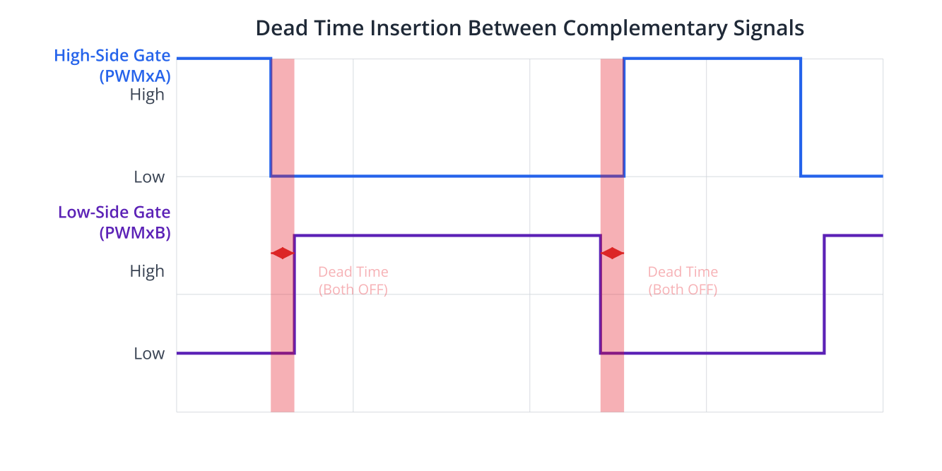
Dead Time Insertion Between Complementary Signals — This timing diagram illustrates how dead time is inserted. During the red-shaded regions, both the high-side and low-side gate signals are OFF, preventing any possibility of shoot-through during the transition.

The ESP32's MCPWM peripheral has a dedicated hardware module to generate this dead time automatically and with high precision, which is a major advantage over trying to implement it in software with delays.

For a more detailed theoretical explanation, the following resource provides an excellent breakdown.

Chapter 164: MCPWM Dead Time and Fault Detection

The article 'MCPWM Dead Time and Fault Detection' from CircuitLabs provides a concise yet thorough explanation of shoot-through and the role of dead time.

Please read the section titled 'Dead Time Insertion', starting from 'What is Shoot-Through?' and ending just before 'MCPWM Dead Time Module'. This will solidify your understanding of the physics and the terminology.

3. From Nanoseconds to Ticks: Calculating Dead Time

To configure the MCPWM peripheral, you can't just tell it "I need 500 nanoseconds of dead time." You must provide the dead time value in terms of the MCPWM timer's ticks. This conversion is a critical step and a common source of error.

Step 1: Find the Required Dead Time from the Datasheet

The required dead time is dictated by the switching characteristics of your MOSFETs. You'll find these values in the MOSFET's datasheet under a section often called "Switching Characteristics" or "Dynamic Characteristics." Look for these key parameters:

Turn-on delay time: $t_{d (o n)}$
Rise time: $t_{r}$
Turn-off delay time: $t_{d (o f f)}$
Fall time: $t_{f}$

The total turn-on time is $t_{d (o n)} + t_{r}$ , and the total turn-off time is $t_{d (o f f)} + t_{f}$ . A safe rule of thumb is to ensure your dead time is longer than the worst-case (maximum) total turn-off time specified in the datasheet.

Dead Time > Max( $t_{d (o f f)} + t_{f}$ )

For example, if a MOSFET datasheet specifies a maximum $t_{d (o f f)}$ of 60 ns and a maximum $t_{f}$ of 40 ns, the total turn-off time is 100 ns. You should choose a dead time safely above this, perhaps 150-200 ns to be conservative.

Step 2: Convert Time to Timer Ticks

Once you have a target dead time in seconds (e.g., 200 ns or $200 \times 1 0^{- 9}$ s), you must convert it to ticks using the timer's resolution you configured previously.

The formula is:

ticks = dead_time_in_seconds \times timer_resolution_hz

Recall from our previous lesson that we configured the timer's resolution:
mcpwm_timer_config_t timer_config = { .resolution_hz = 1000000, ... }; // 1 MHz resolution

So, for a 200 ns dead time and a 1 MHz timer resolution:

ticks = (200 \times 1 0^{- 9}) \times 1, 000, 000 = 0.2

This result highlights a problem: a 1 MHz timer resolution (where 1 tick = 1 µs) is too coarse to specify a dead time in the nanosecond range. To get finer control, you would increase the timer's resolution. For example, if we set .resolution_hz = 10000000 (10 MHz), where 1 tick = 100 ns:

ticks = (200 \times 1 0^{- 9}) \times 10, 000, 000 = 2 ticks

This is a value we can use.

Test your understanding!

You are using an H-bridge with MOSFETs that have a maximum total turn-off time of 450 ns. You've configured your MCPWM timer with a resolution of 8 MHz. To be safe, you want to set a dead time of 600 ns. What integer value should you use for the dead-time ticks in your configuration?

Show answer

The required value is 5 ticks.

First, convert the time to seconds: 600 ns = $600 \times 1 0^{- 9}$ s.
The timer resolution is 8 MHz = $8 \times 1 0^{6}$ Hz.

Using the formula:

ticks = (600 \times 1 0^{- 9}) \times (8 \times 1 0^{6}) = 4800 \times 1 0^{- 3} = 4.8

Since we must provide an integer value for the ticks and need the dead time to be at least 600 ns, we must round up to the nearest integer. Therefore, you should use 5 ticks. This will result in an actual dead time of $5/ (8 \times 1 0^{6}) = 625$ ns, which safely exceeds the 600 ns requirement.

4. Implementation in ESP-IDF

Now, let's put this into code. In the last lesson, we initialized the mcpwm_dead_time_config_t struct but left the delay ticks at zero or used placeholder values. Now we can populate it with our calculated values.

The configuration applies delays to the edges of the primary signal (PWMxA). The complementary signal (PWMxB) is then generated from this delayed and inverted primary signal.

posedge_delay_ticks: The delay applied to the rising edge. This creates dead time before the high-side MOSFET turns ON.
negedge_delay_ticks: The delay applied to the falling edge. This creates dead time before the low-side MOSFET turns ON (since the low-side signal is the inverse of the high-side).

For most H-bridge applications, you will use the same value for both, creating a symmetric dead time.

Here is the relevant code snippet, building upon last lesson's example. This is how you would apply a calculated 2-tick dead time to both rising and falling edges.

#include "esp_log.h"
#include "driver/mcpwm_prelude.h"

// Assume timer, operator, comparator, and generators are already created as in the previous lesson.
// Assume timer resolution is 10 MHz (1 tick = 100 ns)

// Let's set a dead time of 200 ns.
// dead_time_ticks = (200 * 10^-9 s) * (10 * 10^6 Hz) = 2 ticks.
uint32_t dead_time_ticks = 2;

ESP_LOGI(TAG, "Enable dead time of %" PRIu32 " ticks", dead_time_ticks);

// Use the handle for the operator we created earlier
mcpwm_operator_handle_t oper = /* your operator handle */;

mcpwm_dead_time_config_t dt_config = {
    .posedge_delay_ticks = dead_time_ticks,
    .negedge_delay_ticks = dead_time_ticks,
    .flags.invert_output_a = false, // PWMxA is active high (primary)
    .flags.invert_output_b = true,  // PWMxB is active low complementary to PWMxA
};
ESP_ERROR_CHECK(mcpwm_operator_apply_deadtime(oper, &dt_config));

ESP_LOGI(TAG, "MCPWM setup with complementary signals and dead-time is complete.");

This configuration, applied with a single call to mcpwm_operator_apply_deadtime, instructs the hardware to handle all the complex timing for you.

You can find this complete logic within a full example in the circuitlabs.net article.

Chapter 164: MCPWM Dead Time and Fault Detection

The article 'MCPWM Dead Time and Fault Detection' contains a full example that configures complementary PWM with specific dead times. We'll focus on how the dead-time struct is integrated.

Review the code in 'Example 1: Precise Dead-Time Configuration and Verification'. Notice how the mcpwm_dead_time_config_t struct is populated and then applied to the operator after the generators have been created. Also, note the troubleshooting tip in the table below the code about using the correct dead time units (ticks vs. microseconds), which we've just covered.

Conclusion

In this lesson, we took a deep dive into the practical necessity of dead-time insertion for robust H-bridge control. You now understand not just how to enable it, but why it's essential and how to calculate the correct values for your specific hardware.

Key Takeaways:

Shoot-through is a destructive short-circuit condition in an H-bridge caused by the non-instantaneous switching of MOSFETs.
Dead time is a mandatory "both switches off" period that prevents shoot-through.
The ESP32's MCPWM peripheral can generate dead time automatically in hardware, offering high precision.
The required dead time is determined by the MOSFET's turn-off characteristics found in its datasheet.
You must convert the required dead time (in seconds) to timer ticks using the configured timer resolution before passing it to the ESP-IDF.

In our next lesson, we will shift from outputting control signals to processing input signals. We will learn how to configure the PCNT (Pulse Counter) peripheral to read quadrature encoder pulses, which is the fundamental method for getting speed and direction feedback from a motor.

Recommended resources