Dynamic Programming Recurrence Relations

1. The Coin Change Problem: Counting Combinations

Let's start with a classic: the Coin Change problem.

Problem: You are given an array of distinct integer coin denominations and a total amount of money. Your task is to find the number of combinations of coins that make up that amount. You can assume you have an infinite supply of each kind of coin.

For example, if amount = 5 and coins = {1, 2, 3}, how many ways can we form the sum 5?

• 5 = 1 + 1 + 1 + 1 + 1
• 5 = 1 + 1 + 1 + 2
• 5 = 1 + 1 + 3
• 5 = 1 + 2 + 2
• 5 = 2 + 3

The answer is 5.

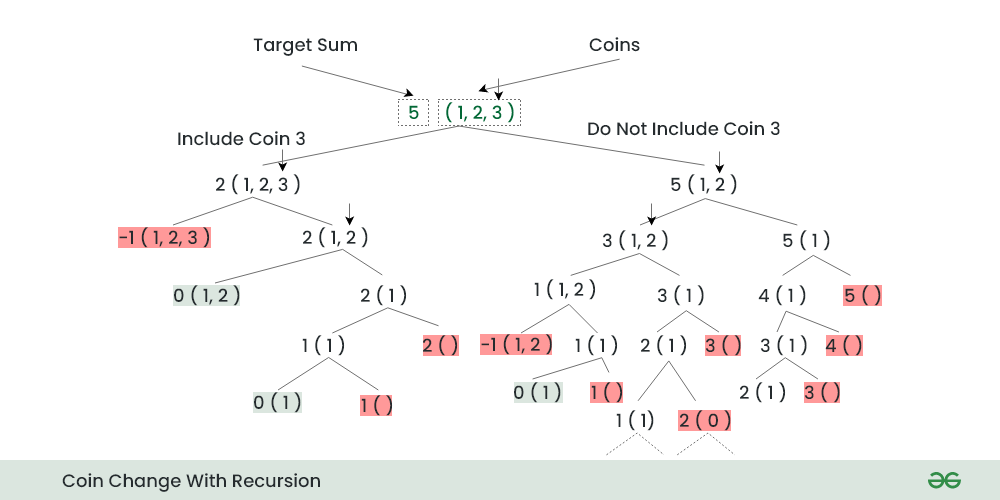
To solve this with DP, we need to break it down. The core idea in many DP problems is to make a decision at each step. Let's consider the coins one by one. For the last coin in our list, say a coin with value c, and a target amount A, we have two choices:

1. Do Not Include Coin c: We decide not to use this coin at all. The problem then reduces to finding the number of ways to make amount A using all the other coins.
2. Include Coin c: We decide to use this coin. After using it once, the remaining amount we need to make is A - c. Crucially, because we have an infinite supply, the problem reduces to finding the number of ways to make this new amount, A - c, still having access to the same set of coins (including c).

This branching decision process can be visualized as a recursion tree.

Formulating the Recurrence

This decision process leads us directly to a recurrence relation. To formalize this, we need to define our DP state. A natural way to capture the subproblem is with two parameters: the coins we are allowed to use, and the amount we need to make.

Let dp[i][a] be the number of ways to make amount a using the first i types of coins (from index 0 to i-1).

Based on our two choices for the $i$-th coin (with value coins[i-1]):

• Case 1 (Do Not Include coin i-1): The number of ways is dp[i-1][a]. We simply solve the same problem with one fewer coin type.
• Case 2 (Include coin i-1): We use one such coin. The remaining amount is a - coins[i-1]. The number of ways to make this remaining amount is dp[i][a - coins[i-1]]. Notice the first parameter is i, not i-1, because we can still use the same coin again.

Since these two cases are mutually exclusive ways to form the total, we add them up. This gives us our state transition equation.

The recurrence is:

This holds if a >= coins[i-1]. If a < coins[i-1], we cannot include the current coin, so dp[i][a] = dp[i-1][a].

2. A Variation: Minimizing the Number of Coins

Let's see how changing the objective affects the recurrence. What if instead of counting combinations, we wanted to find the minimum number of coins to make a certain amount?

This variation still relies on the principle of optimal substructure. This principle states that an optimal solution to a problem is composed of optimal solutions to its subproblems.

Because the problem has optimal substructure, we can build a recurrence. Let's use our 2D state definition again: dp[i][a] is the minimum number of coins to make amount a using the first i coins.

The choices for the $i$-th coin are the same: include it or not.

• Case 1 (Do Not Include coin i-1): The minimum number of coins is dp[i-1][a].
• Case 2 (Include coin i-1): We use one coin (cost: 1) and then need to find the minimum coins for the remaining amount a - coins[i-1]. The total number of coins in this case would be 1 + dp[i][a - coins[i-1]].

Since we want the minimum, we take the minimum of these two options.

The recurrence relation for this new objective is:

Notice the beautiful parallel: we're still choosing between "not including" and "including" the coin. The only things that changed are the combination operator (+ became min) and the value we add when we include a coin (we add the number of combinations dp[...] in the first case, and simply 1 in the second).

3. The Unbounded Knapsack Problem

The Unbounded Knapsack problem is a famous DP problem that perfectly generalizes the structure we've just seen.

Problem: You are given n items, each with a weight and a value. You have a knapsack that can carry a maximum total weight (its capacity). You can take any number of instances of each item. Your goal is to maximize the total value of the items you put in the knapsack.

This problem is called "unbounded" because the supply of each item is infinite, just like our coins. Let's see how the same logic applies.

As the video explains, for any given item i and a remaining knapsack capacity c, our choices are:

1. Do Not Take Item i: We leave the item. The maximum value we can get is found by solving the problem for the first i-1 items with the same capacity c.
2. Take Item i: We put one instance of item i in the knapsack. The value increases by value[i], and the remaining capacity decreases to c - weight[i]. The maximum value we can get from the remaining capacity is found by solving the problem, again with access to the first i items.

Formulating the Recurrence

Let's define our state: dp[i][c] is the maximum value achievable using the first i items with a knapsack capacity of c.

The recurrence relation follows directly from our choices:

The resulting recurrence is:

This formulation should feel very familiar by now. It highlights a powerful pattern for a whole class of "unbounded" problems. The key is always to identify the choice for the current item and correctly express the resulting subproblems.

Conclusion

In this lesson, you took a significant step forward by learning to formulate DP recurrence relations for problems where the state is not tied to a physical grid. You saw how a consistent thought process—breaking the problem down by considering the choices for one item at a time—can be applied to different objectives and constraints.

Key Takeaways:

• Abstract DP States: For problems like Coin Change or Knapsack, the state is often defined by dp[i][amount], representing a solution considering the first i items for a target amount.
• The Core Choice: The recurrence is typically built around two choices for the current item: "include it" or "don't include it."
• Unbounded vs. Bounded: For "unbounded" problems where items can be reused, the "include" case creates a subproblem on the same number of items (dp[i][...]), not one fewer (dp[i-1][...]). This is a critical distinction.
• General Pattern: The structure dp[i][a] = op(dp[i-1][a], value + dp[i][a - size]) is a powerful template, where op can be +, min, max, etc., depending on the problem's goal.

You have now practiced the most important conceptual part of dynamic programming. In our next and final lesson of this module, we will put these recurrences into practice. You will learn how to implement the solutions for Coin Change or Unbounded Knapsack using the bottom-up tabulation method, solidifying your ability to translate DP theory into efficient code.