Dynamic Programming: Coin Change and Unbounded Knapsack (Tabulation)

1. Tabulating the Unbounded Knapsack Solution

Let's begin with the Unbounded Knapsack problem. As a quick reminder, our goal is to maximize the value of items in a knapsack of a given capacity, with an infinite supply of each item. In the last lesson, we derived the following recurrence, where dp[i][c] is the maximum value using the first i items with capacity c:

Tabulation turns this recurrence into an iterative process of filling a 2D array.

Step 1: Setting up the DP Table

We create a 2D table, dp, of size (n + 1) x (capacity + 1), where n is the number of items. Each cell dp[i][c] will store the solution to the corresponding subproblem.

Step 2: Initialization (Base Cases)

The base cases of the recursion become the initial values in our table.

• dp[0][c] = 0 for all c from 0 to capacity. This corresponds to the first row. If we have zero items to choose from, the maximum value we can obtain is always 0, regardless of the knapsack's capacity.
• dp[i][0] = 0 for all i from 0 to n. This corresponds to the first column. If the knapsack has zero capacity, we can't put anything in it, so the value is 0.

Our dp table is typically initialized with all zeros, which conveniently handles both of these base cases.

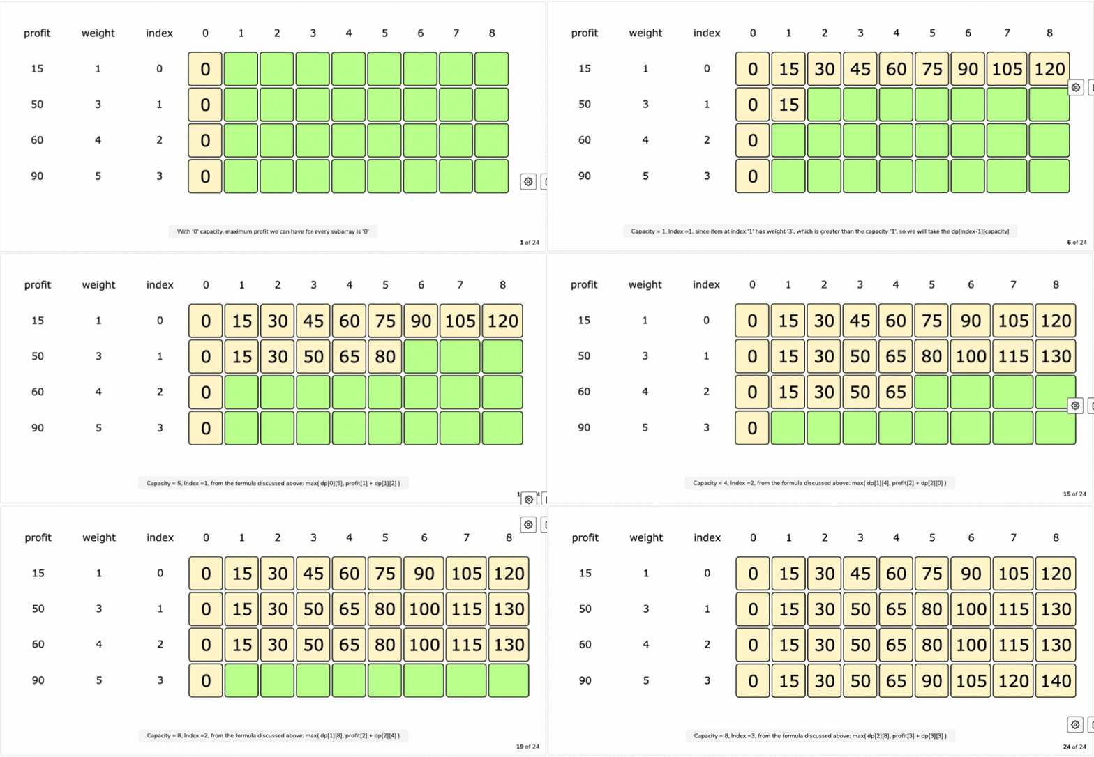
Step 3: Iteration (Filling the Table)

We fill the table iteratively, usually with two nested loops. The outer loop iterates through the items from i = 1 to n, and the inner loop iterates through the capacities from c = 1 to capacity.

Inside the loops, for each cell dp[i][c], we apply our recurrence relation:

1. The "Not Take" case: The maximum value we can get without taking item i-1 is simply the best we could do with the first i-1 items for the same capacity c. This value is already computed and stored in dp[i-1][c].
2. The "Take" case: If the current item's weight (wgt[i-1]) is less than or equal to the current capacity c, we can consider taking it. The value would be val[i-1] plus the maximum value we can get for the remaining capacity, which is c - wgt[i-1]. Crucially, since this is an unbounded problem, we can still use item i-1 again. Therefore, we look up dp[i][c - wgt[i-1]].

The value for dp[i][c] is the maximum of these two options.

The following resource provides a clean C++ implementation of this exact logic.

2. Tabulating the Coin Change Solution

Now let's apply the same principles to the "minimum coins" version of the Coin Change problem. The recurrence we found was:

Here, dp[i][a] is the minimum number of coins to make amount a using the first i coin types.

Step 1: Setup and Initialization

The setup is similar: a 2D table dp of size (num_coins + 1) x (amount + 1). However, the initialization is different and very important.

• dp[i][0] = 0 for all i. It takes 0 coins to make an amount of 0.
• dp[0][a] = \infty for a > 0. With zero coin types available, it's impossible to make any positive amount. We use a large number (like amount + 1, which is an impossible result, or INT_MAX) to represent infinity. This ensures that any valid path will have a smaller value when we use min().

Step 2: Iteration and Implementation

The iteration logic follows the same pattern as the knapsack, but using the Coin Change recurrence. We loop through coins i and amounts a, calculating dp[i][a] as the minimum of not taking the coin (dp[i-1][a]) and taking it (1 + dp[i][a - coins[i-1]]).

The following resource provides an excellent, detailed walkthrough of filling the table for a concrete example.

To see this process in action, the following video segment demonstrates converting the recursive solution into a tabulation solution from scratch, which is a common task in competitive programming.

3. Space Optimization: From 2D to 1D

A O(N * W) space complexity can be too high for problems with large constraints. A key optimization for this class of DP problems is to reduce the space to O(W).

Look at the recurrence for Unbounded Knapsack again:
dp[i][c] = max(dp[i-1][c], ... + dp[i][c - wgt[i-1]])

To compute a value in row i, we only need values from row i-1 (the previous row) and row i (the current row). This suggests we only need two rows at any time. We can do even better and use just a single 1D array.

Let dp[c] be the solution for a capacity c. When we iterate for item i, our update looks like:
dp[c] = max(dp[c], val[i-1] + dp[c - wgt[i-1]])

• The dp[c] on the right side represents the value from the previous iteration (i.e., dp[i-1][c]).
• The dp[c - wgt[i-1]] on the right side needs to be the value from the current iteration (i.e., dp[i][c - wgt[i-1]]).

If we iterate through capacities c in increasing order (a forward loop), when we calculate dp[c], the value dp[c - wgt[i-1]] will have already been updated for the current item i. This is exactly what we need for unbounded problems!

This is a critical distinction from 0/1 Knapsack, where you need values from the previous row only, necessitating a backward loop to avoid using an item more than once.

Now, let's look at the optimized code.

Conclusion

Congratulations on completing the dynamic programming module! You have progressed from the foundational concepts of optimal substructure and overlapping subproblems to implementing robust, optimized solutions for a classic set of DP problems.

Key Takeaways:

• Tabulation is an iterative, bottom-up method that translates a DP recurrence into nested loops that fill a DP table.
• The base cases of the recursion are used to initialize the DP table's first row and/or column.
• The state transition logic is copied into the body of the nested loops to calculate the value of each cell based on previously computed cells.
• For unbounded problems like Unbounded Knapsack and Coin Change, the space can be optimized from a 2D table to a 1D array. This optimization relies on a forward pass in the inner loop to correctly use values updated within the same major iteration.

You have now built a powerful toolkit for solving problems that can be broken down into smaller, reusable parts. This skill is not just a prerequisite for our course, but a cornerstone of advanced algorithm design.

In our next lesson, we will begin a new module that fuses your new DP skills with graph theory. We will introduce Directed Acyclic Graphs (DAGs) and an algorithm called Topological Sort. You will discover how a topological ordering provides a linear path through a graph, allowing us to apply dynamic programming to find shortest and longest paths in a way that would be impossible in general graphs with cycles.