Grid DP: Counting Paths

1. The "Unique Paths" Problem

Let's begin by clearly understanding the problem we aim to solve. Imagine a robot on an m x n grid, starting at the top-left corner and trying to reach the bottom-right corner. The robot is only allowed to move right or down at any point.

As the reading highlights, the key insight is to consider how the robot can arrive at any arbitrary cell (i, j). Since it can only move down or right, it must have come from either the cell directly above, (i-1, j), or the cell directly to the left, (i, j-1). This simple observation is the foundation for our DP solution.

The number of unique paths to (i, j) is therefore the sum of the unique paths to (i-1, j) and the unique paths to (i, j-1). This gives us our recurrence relation.

If we define dp[i][j] as the number of unique paths to reach cell (i, j), the recurrence is:

2. DP States, Transitions, and Base Cases

Before we dive into the code, let's formalize our thinking using some standard DP terminology. You've seen these concepts in action, but defining them explicitly will help you structure your approach to any DP problem.

To summarize for our problem:

• State: The state can be represented by dp[i][j], the number of unique paths to reach cell (i, j). The essential information we need to carry forward is just this count; the specific routes taken to get there are irrelevant for future calculations, which is the core principle of DP.
• Transition: The transition is our recurrence relation, dp[i][j] = dp[i-1][j] + dp[i][j-1]. It defines how we use the solutions of smaller subproblems (reaching (i-1, j) and (i, j-1)) to solve a larger one (reaching (i, j)).
• Base Cases: We need a starting point. For any cell in the first row (i=0), there's only one way to get there: by moving right from the start. Similarly, for any cell in the first column (j=0), there's only one way: by moving down. Therefore, dp[i][0] = 1 and dp[0][j] = 1 for all valid i and j. The most fundamental base case is dp[0][0] = 1.

3. Solving with Tabulation (Bottom-Up)

With the state, transition, and base cases defined, we can now build our solution using tabulation, which is often the most straightforward iterative approach for grid problems. We will create a 2D dp array and fill it out, starting from our base cases.

The process is as follows:

1. Create an m x n 2D array, let's call it dp.
2. Initialize the base cases. A simple way is to set every cell in the first row and first column to 1.
3. Iterate through the rest of the grid, starting from (1, 1). For each cell (i, j), apply the transition: dp[i][j] = dp[i-1][j] + dp[i][j-1].
4. The final answer will be the value in the bottom-right corner, dp[m-1][n-1].

The following image illustrates this process. To find the value for the cell containing '6', we sum the values from the cell above ('3') and the cell to the left ('3').

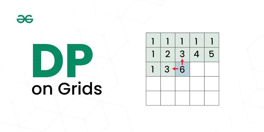
Now, let's see how this logic translates into a full implementation.

This tabulation approach gives us a solution with a time complexity of $O(m\times n)$ because we visit each cell once, and a space complexity of $O(m\times n)$ for the dp table.

4. Alternative: Memoization (Top-Down)

As you know from our previous lessons, we can also solve DP problems using a top-down, recursive approach with memoization. The logic is the reverse of tabulation: we start from the destination (m-1, n-1) and recursively ask "where could I have come from?".

While functionally correct and achieving the same time complexity, this approach uses recursion stack space, which can be a concern in competitive programming for very large grids.

5. Space Optimization

Let's revisit our tabulation recurrence: dp[i][j] = dp[i-1][j] + dp[i][j-1].

Notice that to compute the values for the current row i, we only need the values from the previous row i-1. We don't need rows i-2, i-3, etc. This observation allows for a powerful space optimization, just like we saw with the Fibonacci problem.

Instead of a 2D m x n array, we can use a 1D array of size n. Let's call it prev_row.
When we compute the current_row, current_row[j] will be prev_row[j] (the value from the cell above) + current_row[j-1] (the value from the cell to the left in the current row). After computing the entire current_row, it becomes the prev_row for the next iteration.

We can be even more clever and use just a single 1D array.

This optimization reduces the space complexity from $O(m\times n)$ to $O(n)$ (or $O(\min (m,n))$ if we are smart about which dimension to iterate over), which is a significant improvement for large grids.

Conclusion

In this lesson, we successfully transitioned from 1D to 2D dynamic programming. You learned how to tackle a classic grid-based problem by defining a 2D state, deriving the transition, and handling the base cases.

Key Takeaways:

• 2D DP State: For grid problems, the state dp[i][j] often represents a solution to a subproblem ending at cell (i, j).
• Recurrence on Grids: The recurrence for path-counting is typically dp[i][j] = dp[i-1][j] + dp[i][j-1], summing the results from accessible adjacent cells.
• Tabulation: The bottom-up tabulation approach is a natural fit for grid problems, iterating through the grid and filling the dp table.
• Space Optimization: By analyzing dependencies, we can often reduce space complexity. For this problem, we went from $O(m\times n)$ to $O(n)$ space.

You've added another major DP pattern to your toolkit. In the next lesson, we will explore a different category of DP problems that are not based on grids or simple sequences. We will tackle classic problems like "Coin Change" or "Unbounded Knapsack," where the state definition is less about position and more about abstract quantities.