Hello! Welcome to your fourth lesson in the "Foundations of Clinical Research and Biostatistics" module.
In our last lesson, we tackled the crucial concepts of bias and confounding, learning how they can distort research findings. We established that the first step to good research is a solid study design that minimizes these errors to ensure the data we collect is valid. Now, the question is: once we have this valid data, what do we do with it?
This brings us to the first step of data analysis: describing what we've found. Today's learning outcome is to distinguish between categorical and continuous variables and calculate appropriate descriptive statistics for each.
Mastering this is non-negotiable for your goal of bridging Ayurveda and modern science. Whether you're measuring the effect of ashwagandha on stress levels, classifying patients by their Prakriti, or recording changes in blood markers, you need a systematic language to classify and summarize this information. This lesson provides the fundamental vocabulary and tools for that process.
Part 1: Classifying Your Data - The Types of Variables
Before we can analyze any data, we must first understand its nature. In statistics, the characteristics we measure are called variables. The first and most important classification is whether a variable is categorical or numerical.
Let's watch a video that breaks down these classifications with clear, medically-relevant examples.
Types of Variables - Numerical vs. Categorical - Discrete vs. Continuous - Ordinal vs. Nominal
The video 'Types of Variables' by Medicosis Perfectionalis provides an excellent overview of the main types of variables you will encounter in clinical research.
Watch from 00:29 to 06:19. Focus on understanding the core difference between quantitative (numerical) and qualitative (categorical) variables, and then the subtypes within each category (discrete vs. continuous and nominal vs. ordinal).
As the video explained, we can build a simple hierarchy for data types.
A branching chart showing the types and subtypes of data described in this chapter.
This chart, from the 'College Health Mathematics' resource, provides a clear visual summary of how data (variables) are classified. It starts with the two main branches, Categorical and Numerical, and then shows the sub-types within each.
Let's solidify these definitions:
1. Categorical (Qualitative) Variables
These variables place individuals into groups or categories. They are described with words, not meaningful numbers.
-
Nominal Variables: These are categories with no natural order or ranking.
- Examples: Dosha type (Vata, Pitta, Kapha), blood type (A, B, AB, O), marital status (single, married, widowed). You can't say that "Pitta" is mathematically greater than "Vata".
-
Ordinal Variables: These are categories that have a logical order or rank, but the distance between the categories is not necessarily equal or measurable.
- Examples: A pain scale (e.g., 'mild', 'moderate', 'severe'), patient satisfaction ('poor', 'fair', 'good', 'excellent'), or stages of a disease (Stage I, II, III, IV). We know 'severe' pain is worse than 'mild' pain, but it's not exactly three times worse.
2. Numerical (Quantitative) Variables
These variables are measured on a numeric scale. They represent a quantity.
-
Discrete Variables: These are variables that you can count in whole numbers. There are no "in-between" values.
- Examples: The number of times a patient visits a clinic in a year, the number of herbal tablets prescribed per day, the number of disease relapses. A patient can have 2 or 3 visits, but not 2.5 visits.
-
Continuous Variables: These are variables that can take on any value within a given range. They are measured, not counted.
- Examples: Blood pressure (e.g., 120.5 mmHg), body weight (e.g., 65.7 kg), serum cholesterol levels (e.g., 198.3 mg/dL). There are infinite possibilities between any two values.
To explore these definitions with more health-specific examples, you can refer to the following reading.
Descriptive Statistics – College Health Mathematics
The text 'Descriptive Statistics – College Health Mathematics' provides clear, written definitions and tables with examples relevant to healthcare.
Read the section 'Types of Data', including the subsections on 'Numerical Data' and 'Categorical Data'. Pay attention to the tables that provide examples of each type.
Test your understanding!
Imagine you are conducting a study on the effects of a Panchakarma treatment. For each participant, you record the following information. Classify each variable as Nominal, Ordinal, Discrete, or Continuous.
- Primary Dosha imbalance (Vata, Pitta, or Kapha)
- Age in years
- Symptom severity score before treatment (rated 0=none, 1=mild, 2=moderate, 3=severe)
- Number of previous Panchakarma treatments
- Fasting blood glucose level (in mg/dL)
- Gender (Male, Female, Other)
Show answer
- Nominal: The Dosha types are distinct categories with no inherent numerical order.
- Continuous: While we often report age in whole years, it is technically continuous (a person can be 45.5 years old). It's measured, not counted.
- Ordinal: There is a clear order (severe > moderate > mild), but the difference between the scores is not numerically equal.
- Discrete: You can count the number of treatments in whole numbers (0, 1, 2, etc.).
- Continuous: Blood glucose can be measured to a high degree of precision (e.g., 99.1 mg/dL, 99.2 mg/dL).
- Nominal: These are distinct categories with no ranking.
Part 2: Summarizing Your Data - Descriptive Statistics
Once we've classified our variables, we need to summarize them. This process is called descriptive statistics. Its goal is to provide a simple summary or "snapshot" of our sample data. This is different from inferential statistics (which we'll cover in the next lesson), where we try to make conclusions about a larger population based on our sample.
The following video gives a great overview of descriptive statistics, breaking them down into measures of the "center" of the data and measures of the "spread" of the data.
Descriptive Statistics: FULL Tutorial - Mean, Median, Mode, Variance & SD (With Examples)
This 'Descriptive Statistics: FULL Tutorial' by Grad Coach is a comprehensive yet easy-to-follow guide to the most common descriptive statistics used in research.
Watch the following segments: 00:00 - 02:31: What are descriptive statistics and how do they differ from inferential statistics? 03:47 - 07:10: Measures of central tendency (mean, median, mode). 07:10 - 12:31: Measures of dispersion (range, variance, standard deviation) and a recap. Focus on understanding the concept behind each statistic and when it might be used.
Now, let's detail which statistics are used for which type of variable.
Describing Categorical Data
Summarizing categorical data is straightforward. We use:
- Frequencies (Counts): The number of individuals in each category.
- Proportions (Percentages): The percentage of individuals in each category.
Example: In a study sample of 200 people, you measure their Prakriti.
- Vata: 80 people (40%)
- Pitta: 70 people (35%)
- Kapha: 50 people (25%)
This is typically presented in the text of a paper or in a table. Graphically, it's shown using bar charts or pie charts.
Describing Numerical Data
Summarizing numerical data is more detailed. We use two types of measures:
1. Measures of Central Tendency (Where is the center?)
- Mean: The arithmetic average. To calculate it, you sum all the values and divide by the number of values. The mean is sensitive to outliers (extreme values).
- Median: The middle value when all values are arranged in order. It is not sensitive to outliers, making it a "robust" measure.
- Mode: The value that appears most frequently.
2. Measures of Dispersion (How spread out is the data?)
- Range: The difference between the maximum and minimum value. It's simple but highly affected by outliers.
- Interquartile Range (IQR): The range of the middle 50% of the data. It's calculated as the difference between the 3rd quartile (75th percentile) and the 1st quartile (25th percentile). The IQR is robust to outliers and is often reported along with the median.
- Standard Deviation (SD): This is the most common measure of spread. It tells you the average distance of each data point from the mean. A small SD means the data are clustered tightly around the mean; a large SD means they are spread out. The SD is often reported along with the mean.
Which Descriptive Statistic Should You Use?
This is a critical decision. You can't just calculate everything. The choice depends on the distribution of your data.
- For symmetrical ("normal" or bell-shaped) distributions, the mean and median will be very close. In this case, the mean and standard deviation (SD) are the standard measures to report.
- For asymmetrical (skewed) distributions, outliers will pull the mean in their direction, so it won't represent the "typical" value well. In this case, the median and interquartile range (IQR) are much more appropriate and informative.
Different types of probability distribution
This figure from the 'Basic principles...' article shows how the mean, median, and mode relate in different distributions. In a symmetrical distribution (B), they are all the same. In a skewed distribution (A and C), the mean is pulled towards the long tail, away from the median.
For a deeper dive into these concepts and how to choose the right statistic, this article is an excellent reference.
Basic principles of descriptive statistics in medical research
The article 'Basic principles of descriptive statistics in medical research' provides a concise and practical guide on how to summarize and present data in a medical research context.
Read the sections 'SUMMARIZING CONTINUOUS DATA', 'NUMERICAL AND GRAPHICAL PRESENTATION OF QUALITATIVE DATA', and 'HOW TO CALCULATE AND PRESENT DESCRIPTIVE STATISTICS'. This will reinforce what you've learned and show you how these statistics typically appear in a research paper's 'Table 1'.
Application: Putting It All Together
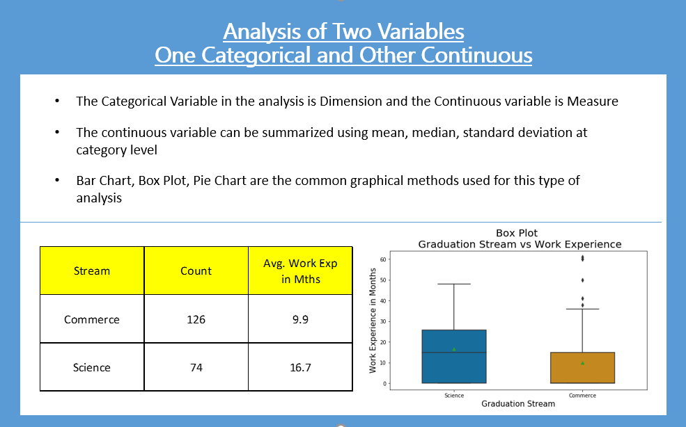
In research, we often analyze a continuous variable across different categories of a categorical variable. For example, we might want to compare the 'change in blood pressure' (continuous) between a 'treatment group' and a 'placebo group' (categorical).
Conclusion
Today, we've laid the essential groundwork for all data analysis. Understanding your data's type and knowing how to properly summarize it is the first step toward drawing meaningful conclusions.
Key Takeaways:
- Variables are either categorical (describing qualities) or numerical (describing quantities).
- Categorical variables can be nominal (unordered) or ordinal (ordered). They are summarized with counts and percentages.
- Numerical variables can be discrete (counted) or continuous (measured). They are summarized using measures of central tendency and dispersion.
- For normally distributed numerical data, use the mean and standard deviation (SD).
- For skewed numerical data, use the median and interquartile range (IQR).
Preview of the Next Lesson:
We now know how to describe the data from our sample. But how do we know if a difference we see in our sample (e.g., the mean blood pressure in the treatment group is 5 mmHg lower than in the placebo group) is a real difference or just due to random chance? To answer that, we need to move from descriptive statistics to inferential statistics. In our next lesson, we will explore the principles of statistical hypothesis testing, including p-values, Type I/II errors, and confidence intervals.