Dropout for Neural Network Regularization

1. The Problem of Overfitting

Imagine you are studying for an exam. You could try to memorize the exact answers to every practice question you're given. You might ace the practice tests, but if the final exam contains slightly different questions, you'd be stuck. A better approach is to understand the underlying concepts, which allows you to solve any related problem.

Overfitting in neural networks is analogous to this memorization strategy. A deep network has enough capacity to create an incredibly complex decision boundary that perfectly separates the training data points, essentially "memorizing" them. This often means it learns the noise in the data, not just the signal.

To prevent this, we introduce regularization, a set of techniques designed to prevent a model from becoming too complex. Today, we focus on dropout.

2. Dropout: The Core Idea

The core idea of dropout is surprisingly simple: during each training step, we randomly "drop out" (i.e., temporarily deactivate) a fraction of the neurons in our network.

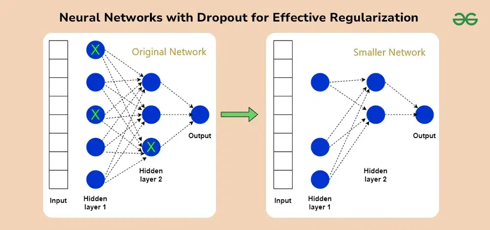
What does this achieve?

1. Ensemble of Models: Each time we drop out a different set of neurons, we are effectively training a different, smaller neural network. Dropout allows us to train an exponential number of these different networks that share weights, and then average their effects, which is a powerful way to reduce overfitting.
2. Prevents Co-adaptation: It stops neurons from becoming too reliant on the presence of other specific neurons. If a neuron knows that its inputs might randomly disappear, it's forced to learn more robust features that are useful on their own, rather than relying on the incidental quirks of its neighbors.

This forces the network to spread out its learning across all its neurons, making the model more robust and less likely to overfit.

3. Implementing Inverted Dropout

While the original dropout paper proposed a specific implementation, the most common method used today is called Inverted Dropout. This technique has a key advantage: it makes the inference (testing) phase much simpler.

Here's how it works during the training phase for a given layer:

1. Define a keep_prob: This is the probability that any given neuron is kept (not dropped). A typical value is 0.5 or 0.8. The dropout rate is 1 - keep_prob.
2. Create a Dropout Mask: Generate a random binary matrix D (the mask) with the same dimensions as the layer's activation output A. Each element in D is set to 1 with probability keep_prob and 0 otherwise.
3. Apply the Mask: Perform an element-wise multiplication of the activations A with the mask D. This zeroes out the activations of the dropped neurons. $$A_{dropped}=A\odot D$$ (where $\odot$ is element-wise multiplication).
4. Scale the Activations: This is the crucial "inverted" step. We scale up the remaining activations by dividing by keep_prob. $$A_{final}=\frac{A_{dropped}}{keep\_prob}$$

Why do we scale?
By dropping neurons, we reduce the expected value of the layer's output. For example, if keep_prob is 0.8, we've zeroed out 20% of the activations, so the sum of the layer's output is roughly 20% smaller. By dividing by 0.8, we scale the remaining activations back up, ensuring that the expected output of the layer remains the same, regardless of the keep_prob value.

This brings us to the inference (testing) phase. Because we already scaled the activations during training, we don't need to do anything special at test time. We simply use the entire network with all neurons active. This is the main benefit of the inverted dropout technique.

4. Code Implementation from Scratch

Now let's translate this into code. Since you've already built forward and backward propagation, we just need to modify those functions. The key is to remember that the same neurons dropped during the forward pass must also be "dropped" during the backward pass. We do this by passing the dropout mask D in the cache.

Let's consolidate the logic into a set of functions. Here's how you would modify forward_propagation and backward_propagation for a simple multi-layer perceptron.

Forward Propagation with Dropout

In the forward_propagation function, after calculating the activation A for a hidden layer, you would add the following steps:

# Assume we have just calculated A1 for the first hidden layer
# keep_prob is a hyperparameter, e.g., 0.8

# 1. Create dropout mask
D1 = np.random.rand(A1.shape[0], A1.shape[1]) < keep_prob

# 2. Apply mask to activations
A1 = A1 * D1

# 3. Scale the activations
A1 = A1 / keep_prob

# Store the mask D1 in the cache along with Z1, A1, etc.
# cache = (..., D1)

You would repeat this for every hidden layer you want to apply dropout to. Dropout is typically not applied to the output layer.

Backward Propagation with Dropout

In backward_propagation, when you are calculating the gradient dA for a layer where you applied dropout, you must re-apply the same mask.

# Assume we have just calculated dA1 for the first hidden layer
# We retrieve D1 from the cache

# Apply the same mask to the gradient
dA1 = dA1 * D1

# Scale the gradient
dA1 = dA1 / keep_prob

# Continue with the rest of backpropagation to calculate dZ1, dW1, db1

By applying the mask D1 to dA1, you ensure that the gradients for the neurons that were dropped during the forward pass are also zeroed out. This is essential for the algorithm to work correctly.

The article also makes an important practical point: when you use a framework like PyTorch or TensorFlow, you must remember to set your model to evaluation mode (e.g., model.eval()) during testing. This automatically disables the dropout layers, so you don't have to manage it manually.

Conclusion

Congratulations! You have now implemented your first regularization technique. By understanding and coding dropout, you've gained a crucial tool for building models that generalize well instead of just memorizing training data.

Key Takeaways:

• Overfitting: Occurs when a model learns the training data too well, including its noise, leading to poor performance on new data.
• Dropout: A regularization technique that randomly deactivates a fraction of neurons during each training step.
• Mechanism: It forces the network to learn more robust, distributed features and acts as a form of model ensembling.
• Inverted Dropout: The standard implementation where activations of remaining neurons are scaled up during training. This simplifies inference, as no changes are needed at test time.
• Implementation: Involves creating and applying a binary mask during forward propagation and then re-applying the same mask to the gradients during backward propagation.

Preview of the Next Lesson:
We've now covered two key aspects of training: optimization (Adam) and regularization (Dropout). There is another powerful technique that addresses a different problem known as "internal covariate shift," which can slow down and destabilize training.

In our next and final lesson of this module, you will implement batch normalization and explain how it stabilizes and accelerates the training process by normalizing the inputs to each layer.