Adam Optimizer: Adaptive Learning Rates

1. From Momentum to Adaptive Learning Rates

Let's quickly recap. Momentum tracks an exponentially weighted moving average of the gradients, which we can call the first moment. This helps determine the direction of our update.

Adam keeps this idea but adds a second, crucial component: an exponentially weighted moving average of the squared gradients, known as the second moment. This will help control the magnitude of our update for each parameter individually.

The intuition is as follows:

• If a parameter's gradients are consistently large, its second moment estimate $v_t$ will be large.
• If a parameter's gradients are small or sparse, its second moment estimate $v_t$ will be small.

Adam uses this second moment to scale the learning rate for each parameter. Specifically, it divides the update by the square root of $v_t$. This means parameters with large historical gradients will get smaller updates (to prevent overshooting), and parameters with small gradients will get larger updates (to make progress). This is the essence of its adaptive learning rate mechanism.

To see how these ideas from Momentum and another optimizer, RMSprop, are combined, let's watch a brief introductory video.

2. The Adam Algorithm: A Step-by-Step Breakdown

Adam is more than just smashing momentum and adaptive rates together. It includes a critical refinement called bias correction. Let's walk through the full algorithm. The Vizuara channel provides an excellent and clear walkthrough of the math and implementation.

Let's formalize the steps from the video. At each training step $t$, for each parameter:

1. Compute Gradient: Calculate the gradient $g_t=\nabla J({\theta }_{t-1})$.
2. Update First Moment (Momentum): $$m_t={\beta }_1{m}_{t-1}+(1-{\beta }_1)g_t$$ This is the momentum term, tracking the mean of the gradients. ${\beta }_1$ is typically 0.9.
3. Update Second Moment (Uncentered Variance): $$v_t={\beta }_2{v}_{t-1}+(1-{\beta }_2)g_t^2$$ This tracks the variance of the gradients. ${\beta }_2$ is typically 0.999.
4. Apply Bias Correction: Since $m_0$ and $v_0$ are initialized to zero, the estimates $m_t$ and $v_t$ are biased toward zero in the initial stages of training. We correct for this bias: $${\hat{m}}_t=\frac{m_t}{1-{\beta }_1^t}\text{and}{\hat{v}}_t=\frac{v_t}{1-{\beta }_2^t}$$
5. Update Parameters: Finally, we update the parameters using the bias-corrected estimates: $${\theta }_t={\theta }_{t-1}-\alpha \frac{{\hat{m}}_t}{\sqrt{{\hat{v}}_t}+ϵ}$$ Here, $\alpha$ is the main learning rate, and $ϵ$ (e.g., $10^{-8}$) is a small value to prevent division by zero.

The term $\frac{\alpha }{\sqrt{{\hat{v}}_t}+ϵ}$ acts as the effective, per-parameter learning rate.

For a more detailed derivation of the bias correction, which is a key theoretical contribution of Adam, the following article is an excellent resource.

3. Implementing Adam from Scratch

Now let's translate the algorithm into code. Your background in Python and previous projects will make this process familiar. We will implement a function that performs the Adam update rule.

The video you watched earlier contains a complete, from-scratch implementation. Additionally, the Machine Learning Mastery article provides a very readable, step-by-step coding guide.

Here is a consolidated Python implementation based on the resources. It performs Adam optimization on a simple quadratic objective function $f(x,y)=x^2+y^2$.

import numpy as np
import matplotlib.pyplot as plt

# Objective function and its derivative
def objective(x, y):
    return x**2.0 + y**2.0

def derivative(x, y):
    return np.array([x * 2.0, y * 2.0])

# Adam optimizer function
def adam(objective_fn, derivative_fn, bounds, n_iter, alpha, beta1, beta2, eps=1e-8):
    # Start at a random point within the bounds
    solution = bounds[:, 0] + np.random.rand(len(bounds)) * (bounds[:, 1] - bounds[:, 0])
    
    # Initialize first and second moment vectors
    m = np.zeros(len(bounds))
    v = np.zeros(len(bounds))
    
    path = [solution.copy()]
    for t in range(1, n_iter + 1):
        # 1. Compute gradient
        g = derivative_fn(solution[0], solution[1])
        
        # 2. Update first moment estimate
        m = beta1 * m + (1.0 - beta1) * g
        
        # 3. Update second moment estimate
        v = beta2 * v + (1.0 - beta2) * g**2
        
        # 4. Compute bias-corrected estimates
        m_hat = m / (1.0 - beta1**t)
        v_hat = v / (1.0 - beta2**t)
        
        # 5. Update parameters
        solution -= alpha * m_hat / (np.sqrt(v_hat) + eps)
        
        path.append(solution.copy())
        
    return path

# --- Hyperparameters ---
bounds = np.asarray([[-1.0, 1.0], [-1.0, 1.0]])
n_iter = 100
alpha = 0.02
beta1 = 0.8
beta2 = 0.999

# --- Run and Plot ---
path_adam = adam(objective, derivative, bounds, n_iter, alpha, beta1, beta2)
path_adam = np.array(path_adam)

# You can run this code locally to visualize the optimization path
# The path will show a much more direct and rapid convergence than simple SGD
print(f"Adam finished. Final point: {path_adam[-1]}")

Notice how each line in the loop directly maps to the five steps of the algorithm we defined. This small amount of code encapsulates a powerful optimization strategy that is the backbone of training for many modern neural networks.

4. Why is Adam so Widely Used?

Adam's combination of momentum and adaptive learning rates makes it incredibly effective and robust.

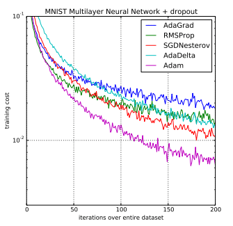
The key benefits are:

• Fast Convergence: It often finds the minimum of the loss function much faster than other optimizers.
• Robustness: It is less sensitive to the choice of the learning rate ($\alpha$) than SGD. The default hyperparameters ($\alpha =0.001,{\beta }_1=0.9,{\beta }_2=0.999$) work well for a surprisingly wide range of models.
• Memory Efficiency: It requires little memory, as it only needs to store the first and second moment vectors, which are the same size as the parameter gradients.

Conclusion

Congratulations! You have now mastered one of the most important algorithms for training deep neural networks. By understanding how Adam works from first principles and implementing it yourself, you have gained a deep insight that goes far beyond simply calling a library function.

Key Takeaways:

• Core Idea: Adam combines momentum (first moment of gradients) to determine update direction with an adaptive learning rate mechanism (second moment of gradients) to scale the update magnitude for each parameter.
• Adaptive Mechanism: It divides the learning rate by a moving average of squared gradients ($v_t$). This gives smaller updates to parameters with large, consistent gradients and larger updates to those with small or sparse gradients.
• Bias Correction: Adam corrects for the initial zero-bias of its moment estimates, making it reliable from the very first training steps.
• Implementation: The algorithm involves five steps: compute gradient, update first moment, update second moment, apply bias correction, and update parameters.

Preview of the Next Lesson:
So far, we have focused entirely on making our model train faster and more effectively. But what if our model gets too good at learning the training data? It might start to memorize the examples, including their noise, and fail to perform well on new, unseen data. This problem is called overfitting.

In our next lesson, we will begin tackling this issue by exploring our first regularization technique. You will implement dropout regularization and explain how it prevents overfitting by randomly "turning off" neurons during training, forcing the network to learn more robust features.