Batch Normalization: Stabilizing Neural Network Training

1. The Problem: Internal Covariate Shift

Let's visualize the problem. Many activation functions, like the sigmoid or tanh, have "saturated" regions where their gradient is close to zero. If the inputs to these functions fall into these regions, the gradients vanish, and learning grinds to a halt. Internal covariate shift can push the activations into these undesirable regions as the network trains.

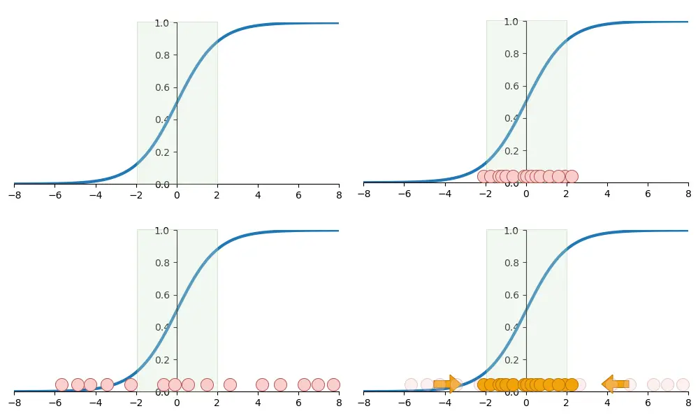
The core idea of Batch Normalization (BN), introduced in 2015, is elegantly simple: if the shifting distributions are the problem, why not explicitly force the inputs to each layer to have a stable distribution throughout training?

2. The Core Idea of Batch Normalization

Batch Normalization normalizes the output of a previous layer before it's fed into the next one. For each mini-batch during training, and for each feature/neuron independently, it performs the following steps:

This process ensures that the inputs to the next layer are always centered around a mean of 0 and have a standard deviation of 1, regardless of what's happening in the preceding layers.

To get a better sense of why this is so effective, let's start with a video that outlines the main benefits.

3. Forward Pass: The Mechanics

While forcing the activations to a standard Gaussian distribution (mean 0, variance 1) seems like a good idea for stability, it might be too restrictive. What if the optimal representation for a layer actually requires a different mean and variance?

To solve this, Batch Normalization introduces two learnable parameters per feature:

1. A scale parameter, $\gamma$ (gamma), initialized to 1.
2. A shift parameter, $\beta$ (beta), initialized to 0.

After normalization, the layer's output is scaled by $\gamma$ and shifted by $\beta$.

Here, ${\hat{x}}_i$ is the normalized activation. Since $\gamma$ and $\beta$ are learnable, the network can decide the optimal mean and variance for each layer's inputs. In a worst-case scenario, it can learn $\gamma =\sqrt{{\sigma }_{\mathcal{B}}^2}$ and $\beta ={\mu }_{\mathcal{B}}$, effectively undoing the normalization and recovering the original activations. This means BN can't hurt the network's representational power.

Training vs. Inference

A crucial detail of Batch Normalization is that it behaves differently during training and inference.

• During training, we normalize using the current mini-batch's mean and variance. This is fine because we process data in batches.
• During inference (testing), we might want to process a single example. Calculating a "batch" mean and variance for a single sample is meaningless. Furthermore, we want our model's output to be deterministic for a given input, not dependent on other examples in a hypothetical batch.

The solution is to calculate an exponential moving average of the batch means and variances during training. These running statistics provide a stable estimate of the entire training set's statistics. At inference time, we use these fixed running averages to normalize the inputs.

Let's watch a detailed walkthrough of this process.

4. Implementation from Scratch

Now let's consolidate everything into a Python class. We will implement the forward pass with two modes: 'train' and 'test' (or 'eval').

Below is a NumPy-based implementation of the BatchNorm forward pass. Note how it mirrors the logic from the resources you've just studied.

import numpy as np

class BatchNorm1d:
    def __init__(self, num_features, eps=1e-5, momentum=0.9):
        # Learnable parameters
        self.gamma = np.ones(num_features)  # scale
        self.beta = np.zeros(num_features) # shift

        # Parameters for inference mode
        self.running_mean = np.zeros(num_features)
        self.running_var = np.ones(num_features)
        
        # Hyperparameters
        self.eps = eps
        self.momentum = momentum
        self.training = True # Controls mode
        
        # Cache for backward pass
        self.cache = None

    def forward(self, x):
        # x is the input, shape (batch_size, num_features)
        
        if self.training:
            # 1. Calculate batch mean and variance
            batch_mean = np.mean(x, axis=0)
            batch_var = np.var(x, axis=0)

            # 2. Normalize the batch
            x_hat = (x - batch_mean) / np.sqrt(batch_var + self.eps)

            # 3. Update running statistics for inference
            self.running_mean = self.momentum * self.running_mean + (1 - self.momentum) * batch_mean
            self.running_var = self.momentum * self.running_var + (1 - self.momentum) * batch_var
            
            # Store values needed for backward pass
            self.cache = (x, x_hat, batch_mean, batch_var, self.gamma)
        else:
            # At inference, use running statistics
            x_hat = (x - self.running_mean) / np.sqrt(self.running_var + self.eps)
        
        # 4. Scale and shift
        out = self.gamma * x_hat + self.beta
        return out

5. Backward Pass: The Gradients

The backward pass for Batch Normalization is more complex than for other layers we've seen. This is because the output for each sample in a batch depends not only on its corresponding input but on all other samples in the batch through the shared batch mean and variance.

This inter-dependency means the gradient calculation must account for how a single input $x_i$ affects the loss through all outputs in the batch. While the derivation is an excellent exercise in applying the chain rule, we will focus on the intuition and the final implementation.

Here is the implementation of the backward method, which you can add to our BatchNorm1d class. It uses the values stored in self.cache from the forward pass.

    def backward(self, dout):
        # dout is the upstream gradient from the next layer
        x, x_hat, batch_mean, batch_var, gamma = self.cache
        N, D = x.shape

        # Gradient of learnable parameters (dgamma, dbeta)
        self.dbeta = np.sum(dout, axis=0)
        self.dgamma = np.sum(dout * x_hat, axis=0)

        # Gradient with respect to the input x (dx)
        # This is the most complex part of the backprop
        
        # 1. Gradient of loss w.r.t. normalized output
        dx_hat = dout * gamma
        
        # 2. Gradient of loss w.r.t. variance
        dvar = np.sum(dx_hat * (x - batch_mean) * -0.5 * (batch_var + self.eps)**(-1.5), axis=0)
        
        # 3. Gradient of loss w.r.t. mean
        dmean = np.sum(dx_hat * -1 / np.sqrt(batch_var + self.eps), axis=0) + \
                dvar * np.sum(-2 * (x - batch_mean), axis=0) / N
        
        # 4. Gradient of loss w.r.t. input x
        dx = (dx_hat / np.sqrt(batch_var + self.eps)) + \
             (dvar * 2 * (x - batch_mean) / N) + \
             (dmean / N)
        
        return dx

6. Mapping to PyTorch

Understanding the from-scratch implementation gives you a huge advantage when using high-level frameworks like PyTorch. The concepts map directly. Our BatchNorm1d class is a simplified version of PyTorch's nn.BatchNorm1d.

Conclusion

Congratulations on completing the "Neural Network Foundations" module! You've gone from the fundamentals of backpropagation to implementing some of the most important optimizers and regularizers used in modern deep learning.

Key Takeaways from this Lesson:

• Problem: Internal Covariate Shift destabilizes and slows down training by constantly changing the input distributions to layers.
• Solution: Batch Normalization standardizes the inputs to each layer for every mini-batch, forcing them to have a mean of 0 and a variance of 1.
• Representational Power: Learnable scale ($\gamma$) and shift ($\beta$) parameters are added to allow the network to learn the optimal distribution for each layer.
• Training vs. Inference: BN uses batch statistics during training but relies on fixed running averages of mean and variance for deterministic output during inference.
• Effect: BN stabilizes training, which allows for much higher learning rates, faster convergence, and acts as a mild regularizer.

Preview of the Next Module:
You have built an incredible foundation by implementing these concepts from scratch. You now understand not just what these layers do, but how they work under the hood.

In our next module, "Applied Deep Learning in PyTorch," we will leverage this deep understanding to build and train models more efficiently using the powerful and optimized building blocks provided by PyTorch. We'll start by building our first feedforward network in PyTorch and training it on a real classification task.