Forward Pass: MLP Output Calculation

Hello! Welcome to your second lesson.

In our previous session, we defined the fundamental components of a neural network: the neuron and the Multi-Layer Perceptron (MLP). We established that the computation for an entire layer can be expressed with the compact and powerful equation: $h = ϕ (Wx + b)$ .

Today, we will put that equation to work. Our goal is to compute the final output of an MLP for a given input vector. This process of passing an input through the network layer by layer is known as the forward pass or forward propagation. Mastering this is essential, as it's the core operation performed repeatedly within every block of the transformer models we are working towards.

1. The Forward Pass: A Chain of Transformations

An MLP computes its output by composing functions. The output of the first layer becomes the input to the second, the output of the second becomes the input to the third, and so on, until the final layer produces the network's prediction.

Let's formalize this with the notation from our last lesson:

The initial input vector is $x$ .
The activation of the first hidden layer is: $h^{(1)} = ϕ_{1} (W^{(1)} x + b^{(1)})$
The activation of the second hidden layer, which takes $h^{(1)}$ as its input, is: $h^{(2)} = ϕ_{2} (W^{(2)} h^{(1)} + b^{(2)})$
This continues until the final output layer: $y = ϕ_{o u t} (W^{(o u t)} h^{(L)} + b^{(o u t)})$ , where $L$ is the last hidden layer.

The following reading provides a concise summary of this sequential process.

Neural Networks From Linear Algebraic Perspective

Let's start with a formal overview of the forward pass. This article, 'Neural Networks From Linear Algebraic Perspective,' lays out the process clearly.

Read the section 'Neural Network 101'. Focus on how Equation 1(a) and Equation 1(b) are chained together to form the complete forward pass. This demonstrates the step-by-step flow of data through the network.

The entire network, no matter how deep, is just one large composite function that transforms an input vector into an output vector. The "intelligence" of the network is encoded in the values of the weight matrices ( $W$ ) and bias vectors ( $b$ ).

2. A Practical Walkthrough of the Forward Pass

Now, let's dive into the mechanics. How do we efficiently compute $Wx + b$ for an entire layer? The key is to leverage matrix and vector operations, which are highly optimized in deep learning libraries.

This first video provides a fantastic, step-by-step guide to building the forward pass computation, starting from a single neuron and scaling up to a full layer.

Vectorize BackProp Tutorial: Forward Pass

The video 'Vectorize BackProp Tutorial: Forward Pass' by Ryan Harris offers a clear, practical explanation of how to implement the forward pass using vectorized operations.

Watch from 01:16 to 09:22. The video breaks this down into several key steps: Handling the Bias (01:16 - 04:12): Notice the practical trick of adding a 'bias node' that always outputs 1. This allows the bias term to be incorporated into the weight matrix, simplifying the equation to a single matrix-vector multiplication. This is a common implementation detail. From One Neuron to a Layer (04:12 - 07:50): See how the calculation for a single neuron's input naturally expands to calculating the inputs for all neurons in the layer simultaneously using a single matrix-vector product. Applying Activation (07:50 - 09:22): Understand that after the linear transformation (Wx + b), a non-linear activation function is applied element-wise to get the layer's final output, which is then ready to be fed into the next layer.

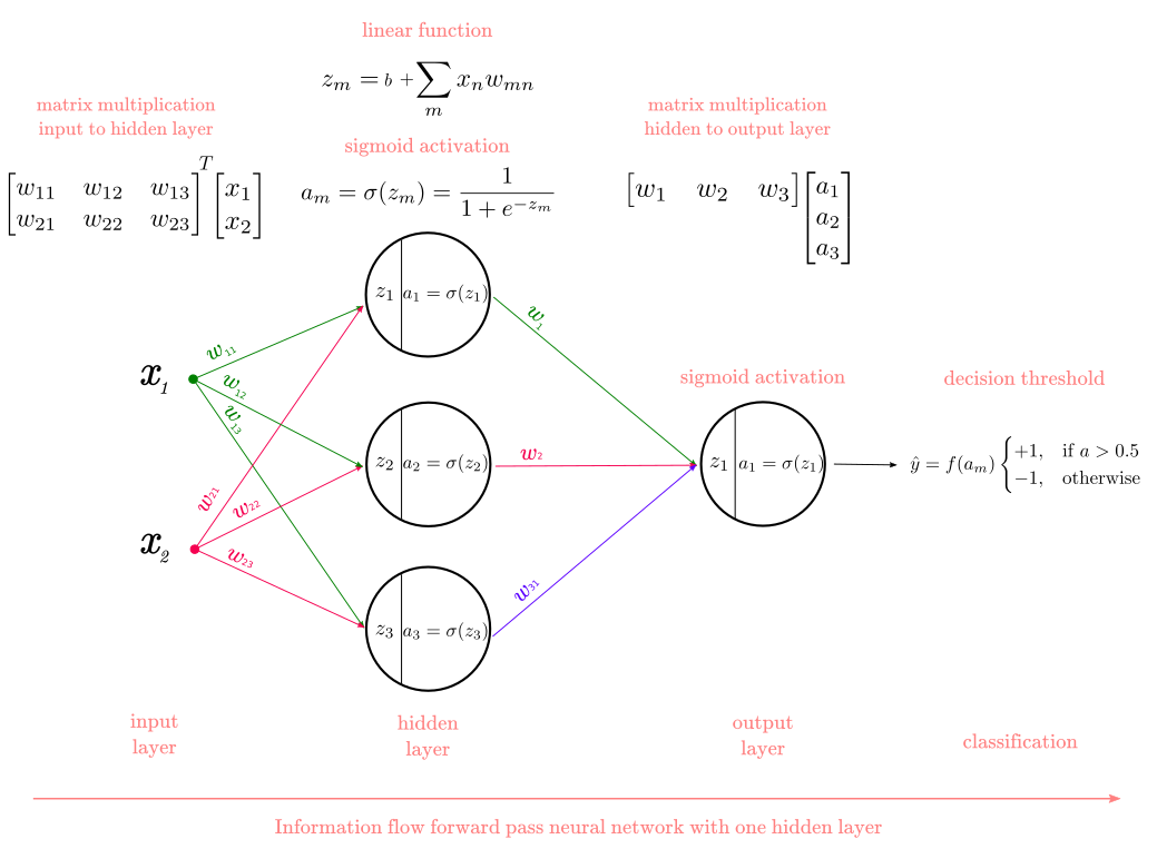
To summarize the process for computing the output of one layer given an input vector $x$ :

Define the layer's parameters:
- A weight matrix $W$ , where the number of rows is the number of neurons in the current layer, and the number of columns is the number of neurons in the previous layer (or the size of the input vector).
- A bias vector $b$ with a size equal to the number of neurons in the current layer.
Perform the affine transformation: Calculate $z = Wx + b$ . This is a matrix-vector multiplication followed by a vector addition. The result $z$ is often called the pre-activation or logit.
Apply the non-linear activation: Calculate the layer's output (its activations) $h$ by applying the activation function $ϕ$ to each element of $z$ : $h = ϕ (z)$ .

You then repeat these three steps for every layer in the network.

Forward Pass in a Single Hidden Layer Neural Network — This diagram shows the complete forward pass for a simple network. The input `x` is transformed by the first layer's weights `W_h` and bias `b_h` to get `z_h`, which is then passed through a sigmoid activation to get `a_h`. This process is repeated for the output layer.

Test your understanding!

Let's compute a forward pass for a small MLP by hand. The network has 2 input neurons, a hidden layer with 2 neurons, and 1 output neuron. The activation function for both layers is ReLU ( $ϕ (z) = max (0, z)$ ).

The parameters are:

Input vector: $x = [0.5 - 1]$
Hidden layer weights and bias:
$W^{(1)} = [1 - 2 23], b^{(1)} = [0 - 1]$
Output layer weights and bias:
$W^{(2)} = [4 - 1], b^{(2)} = [2]$

Calculate the final output of the network, $y$ .

Show answer

First Layer (Input to Hidden):
- Compute the pre-activation $z^{(1)}$ :
  $z^{(1)} = W^{(1)} x + b^{(1)} = [1 - 2 23] [0.5 - 1] + [0 - 1]$
  $= [(1 \cdot 0.5) + (2 \cdot - 1) (- 2 \cdot 0.5) + (3 \cdot - 1)] + [0 - 1] = [- 1.5 - 4] + [0 - 1] = [- 1.5 - 5]$
- Apply the ReLU activation function to get $h^{(1)}$ :
  $h^{(1)} = ReLU (z^{(1)}) = [max (0, - 1.5) max (0, - 5)] = [00]$
Second Layer (Hidden to Output):
- Compute the pre-activation $z^{(2)}$ , using $h^{(1)}$ as the input:
  $z^{(2)} = W^{(2)} h^{(1)} + b^{(2)} = [4 - 1] [00] + [2]$
  $= [(4 \cdot 0) + (- 1 \cdot 0)] + [2] = [0] + [2] = [2]$
- Apply the ReLU activation to get the final output $y$ :
  $y = ReLU (z^{(2)}) = [max (0, 2)] = [2]$

The final output of the network is 2.

3. Scaling Up: Processing Data in Batches

In real-world applications, from data analytics to training LLMs, we never process a single data point at a time. It is far more efficient to process a "batch" of inputs simultaneously. Your background in data analytics has likely made you familiar with the concept of operating on entire columns or matrices of data at once, and neural networks are no different.

The beauty of the matrix formulation is that it scales seamlessly from a single input vector to a matrix of many input vectors. Instead of an input vector $x$ , we have an input matrix $X$ , where each column (or row, depending on convention) is a separate input example. The math remains the same: a single matrix-matrix multiplication processes the entire batch.

Let's see how this works.

Vectorize BackProp Tutorial: Forward Pass

This final clip from the same video explains this crucial optimization. It shows how to arrange multiple input examples into a matrix to perform a forward pass for all of them in a single, efficient operation.

Watch from 09:22 to 12:37. The key insight here is how stacking input vectors into a matrix X allows you to compute the outputs for all of them with a single matrix-matrix multiplication. This is a cornerstone of efficient deep learning code and leverages the full power of modern hardware (like GPUs).

To formalize this, let's adopt the common convention where the batch of inputs is a matrix $X$ of size m x n_in, where m is the batch size (number of examples) and n_in is the number of features.

The forward pass for a batch then looks like this:

Layer 1:
- Weights $W^{(1)}$ have shape n_in x n_hid.
- Bias $b^{(1)}$ has shape 1 x n_hid.
- Pre-activation: $Z^{(1)} = X W^{(1)} + b^{(1)}$ . The bias vector $b^{(1)}$ is broadcast across each of the m rows. The resulting matrix $Z^{(1)}$ has shape m x n_hid.
- Activation: $H^{(1)} = ϕ (Z^{(1)})$ .
Layer 2:
- The activation matrix $H^{(1)}$ is the input to the next layer. The process repeats.

This batch-based computation is fundamental to training neural networks efficiently.

Conclusion

In this lesson, we demystified the forward pass, the process of computing a neural network's output.

Key Takeaways:

The forward pass is a sequence of transformations, where the output of one layer becomes the input for the next.
For each layer, the computation consists of an affine transformation ( $Wx + b$ ) followed by an element-wise non-linear activation ( $ϕ$ ).
Using matrix operations allows us to compute the transformations for an entire layer—and even an entire batch of data—in a single, efficient step. This vectorization is key to the performance of modern deep learning.

You now understand how to get a prediction from a known network. But how do we know if that prediction is correct? And if it's wrong, how do we adjust the network's 13,000+ parameters (as in the 3Blue1Brown example) to make it better?

In the next lesson, we will introduce the concept of a loss function, a way to mathematically quantify the error in your network's predictions. This will be the first step on our journey toward understanding how neural networks learn.

Recommended resources

1. The Forward Pass: A Chain of Transformations

2. A Practical Walkthrough of the Forward Pass

3. Scaling Up: Processing Data in Batches

Conclusion