Loss Functions: Quantifying Prediction Error

1. From Raw Outputs to Probabilities: The Softmax Function

The forward pass ends with a vector of raw numerical values, often called logits. For a classification task (e.g., predicting the next word in a sentence from a vocabulary of 50,000 words), these raw scores aren't very useful. We need to convert them into a set of probabilities, where each value is between 0 and 1, and all values sum to 1.

This is the job of the Softmax function. It takes a vector of $K$ real numbers and normalizes it into a probability distribution over $K$ possible outcomes.

The video below gives a clear explanation of how the final layers of a neural network produce these probabilities.

Mathematically, if our network produces a logit vector $\mathbf{z}=[z_1,z_2,...,z_K]$, the Softmax function calculates the $i$-th component of the output probability vector $\hat{\mathbf{y}}$ as:

${\hat{y}}_i=\text{Softmax}(\mathbf{z}{)}_i=\frac{e^{z_i}}{{\sum }_{j=1}^K{e}^{z_j}}$

The exponential function, $e^{z_i}$, ensures all output values are positive. Dividing by the sum of all these exponentiated values ensures that the final probabilities sum to 1. Now, our network's output $\hat{\mathbf{y}}$ is a valid probability distribution, which we can compare to the true distribution.

2. Quantifying Error with Information Theory

How do we measure the "error" between our predicted probability distribution ($\hat{\mathbf{y}}$) and the true distribution ($\mathbf{y}$)? We can find a powerful answer in the field of information theory.

The key idea is surprise. Intuitively, if a very unlikely event occurs, we are more surprised than if a very likely event occurs. Information theory quantifies surprise for an event with probability $p$ as $-\log (p)$.

From this, we can define cross-entropy, which measures the average surprise we experience when observing events from a true probability distribution $P$, while our beliefs about their likelihood are described by a different distribution $Q$. This is precisely our scenario: we observe the real world (distribution $P$) while using our model's predictions (distribution $Q$) to estimate probabilities.

The following video masterfully builds these concepts from the ground up.

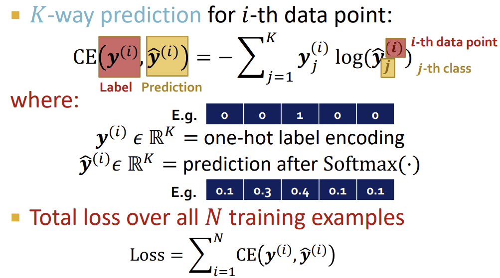
The mathematical formula for the cross-entropy between a true discrete distribution $P$ and a model's predicted distribution $Q$ is:

$H(P,Q)=-{\sum }_{i=1}^{K}P(i)\log (Q(i))$

Here, $K$ is the number of possible classes or outcomes. This formula calculates a weighted average of the surprise ($-\log (Q(i))$) for each outcome, where the weights are the true probabilities $P(i)$. Our goal in training a neural network will be to adjust its parameters to make this cross-entropy value as small as possible.

3. Cross-Entropy as a Neural Network Loss Function

Let's now apply this formal definition directly to our neural network. In a typical classification problem:

• The true distribution $P$ is represented by a one-hot vector $\mathbf{y}$. For example, if we have 5 classes and the correct class is the 3rd one, then $\mathbf{y}=[0,0,1,0,0]$. This means $P(3)=1$ and $P(i)=0$ for all other $i$.
• The predicted distribution $Q$ is the output of our Softmax layer, $\hat{\mathbf{y}}$.

Because the true distribution vector $\mathbf{y}$ is all zeros except for a single 1 at the correct class index (let's call it $c$), the big sum in the cross-entropy formula collapses into a single term:

$H(\mathbf{y},\hat{\mathbf{y}})=-{\sum }_{i=1}^K{y}_i\log ({\hat{y}}_i)=-y_c\log ({\hat{y}}_c)=-\log ({\hat{y}}_c)$

This beautifully simple result is the negative log probability of the correct class. It has a powerful and intuitive meaning: to minimize the loss, the network must learn to maximize the probability it assigns to the correct answer. This is also known as maximizing the log-likelihood of the data, a concept you might have encountered in statistical modeling.

The following video connects these pieces and shows why cross-entropy and negative log-likelihood are, in this context, the same objective.

The behavior of this loss function is exactly what we want. Look at the plot below for a binary classification task (two outcomes, 0 or 1).

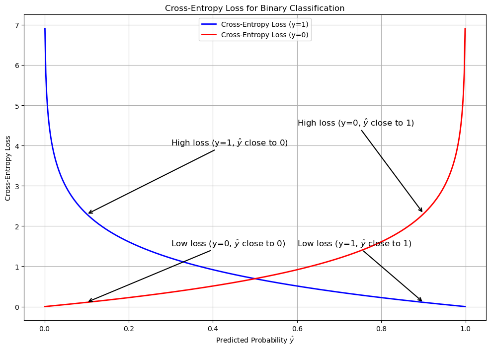
As you can see, the loss penalizes the model heavily for being confident and wrong (e.g., predicting 0.01 when the answer is 1 results in a very high loss), while rewarding it for being confident and correct.

4. Why Cross-Entropy? The Link to KL Divergence

You might be wondering if other loss functions could work. Why is cross-entropy so prevalent? The final piece of the puzzle lies in its relationship to another information-theoretic measure: Kullback-Leibler (KL) Divergence.

KL Divergence, $D_{KL}(P||Q)$, measures the "extra surprise" you get from using distribution $Q$ to model distribution $P$. It's a direct measure of how much information is lost when $Q$ is used to approximate $P$. Our goal in training is to find a model $Q$ that is as close as possible to the true data distribution $P$, which means we want to minimize $D_{KL}(P||Q)$.

The relationship between KL Divergence and Cross-Entropy is simple and profound:
$D_{KL}(P||Q)=H(P,Q)-H(P)$
Where $H(P,Q)$ is the cross-entropy and $H(P)$ is the entropy of the true distribution $P$.

In a machine learning task, the true data distribution $P$ is fixed. We can't change it. This means its entropy, $H(P)$, is a constant. Therefore, minimizing the KL Divergence is mathematically equivalent to minimizing the cross-entropy. Since cross-entropy is easier to compute, it becomes our practical optimization objective.

Conclusion

In this lesson, we have built the crucial bridge between making a prediction and evaluating it. We've established a principled, mathematically sound method for quantifying our model's error.

Key Takeaways:

• A loss function computes a numerical score that represents the error between a model's prediction and the ground truth.
• The Softmax function is used to convert the raw output logits of a classifier into a valid probability distribution.
• Cross-entropy loss is derived from information theory and measures the "average surprise" when comparing the model's predicted distribution to the true distribution.
• For classification, cross-entropy simplifies to the negative log-likelihood of the correct class. Minimizing this loss encourages the model to assign a high probability to the correct answer.
• Optimizing for cross-entropy is equivalent to minimizing the KL Divergence between the model's distribution and the true data distribution, which is the ultimate goal of training.

We now have a complete forward path: an input goes in, a prediction comes out, and a single number—the loss—tells us how good that prediction was. The entire network is just one giant, differentiable function.

This leads to the final, most important question: How do we use this loss value to systematically update the millions of weights and biases in the network to improve its performance? That is the subject of our next and final lesson in this module: backpropagation and gradient descent.