Artificial Neurons and MLPs: Mathematical Foundations

Hello! Welcome to the first lesson in our course on the architecture of Large Language Models.

Your goal is to understand the mathematical foundations of modern transformer models. To get there, we must start with the fundamental building block of all deep learning: the artificial neuron. This lesson will define the mathematical structure of a single neuron and then show how these neurons are combined into a Multi-Layer Perceptron (MLP), which forms a core component within the larger transformer architecture.

By the end of this lesson, you will be able to define the mathematical structure of an artificial neuron and a multi-layer perceptron. This foundation is essential for everything that follows.

1. What is an Artificial Neuron?

At its core, a neural network is a collection of interconnected computational units called neurons. While inspired by the brain, the artificial neuron is a much simpler mathematical construct. It takes one or more numerical inputs, processes them, and produces a single numerical output.

To get a high-level intuition, let's start with a video from the excellent 3Blue1Brown series.

But what is a neural network? Chapter 1, Deep learning

This video, titled 'But what is a neural network?', provides a fantastic visual introduction to the concepts of neurons and layers. Please watch the first part, which introduces the idea of a neuron as a number-holder and the layered structure of a network.

Starting around two minutes and forty seconds in, watch the network structure. Focus on how the network is structured into an input layer, hidden layers, and an output layer, and the idea that a neuron's 'activation' is just a number.

As the video explains, a neuron's job is to compute an output value (its activation) based on the inputs it receives from the previous layer. This computation involves three key components: weights, a bias, and an activation function.

Let's break down the process for a single neuron:

Weighted Sum: The neuron receives multiple inputs, let's call them $x_{1}, x_{2}, \dots, x_{n}$ . Each input connection has an associated weight ( $w_{1}, w_{2}, \dots, w_{n}$ ). The neuron calculates a weighted sum of its inputs: $z = (w_{1} x_{1} + w_{2} x_{2} + \dots + w_{n} x_{n})$ . The weights are the primary parameters the network learns; they determine the importance of each input.
Bias: A bias ( $b$ ) is added to this weighted sum: $z = (w_{1} x_{1} + \dots + w_{n} x_{n}) + b$ . The bias is another learnable parameter that can shift the output independently of the inputs, effectively making the neuron easier or harder to activate.
Activation Function: The result $z$ is then passed through a non-linear activation function, $ϕ$ , to produce the final output, or activation, of the neuron: $a = ϕ (z) = ϕ (\sum_{j} w_{j} x_{j} + b)$ .

The video you just watched explains this process clearly. Let's continue with it to see how weights, biases, and the activation function come together.

But what is a neural network? Chapter 1, Deep learning

This next segment from the same 3Blue1Brown video explains the roles of weights and biases in detail and introduces a common activation function, the sigmoid function.

Starting around 8 minutes in, watch the activation mechanism. Pay close attention to how weights and biases are used to control the neuron's output and how the sigmoid function 'squishes' the result into a range between 0 and 1.

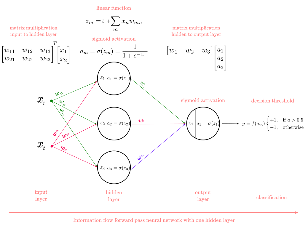
The sigmoid function, $σ (z) = \frac{1}{1 + e ^{- z}}$ , is historically important. It maps any real-valued number to the range (0, 1), which was convenient for interpreting neuron activations as probabilities or firing rates.

This diagram illustrates the flow of information for a single neuron. The inputs $x_i$ are multiplied by weights $w_i$, summed with a bias $b$, and then passed through an activation function (here, sigmoid $\sigma$) to produce the neuron's output activation $a$.

2. The Importance of Non-Linearity

Why bother with an activation function? If we omitted it, the neuron's output would simply be $a = z = \sum w_{j} x_{j} + b$ , which is a linear function of the inputs. If you stack layers of linear functions, the entire network would still only be able to compute a single, complex linear function. A composition of linear functions is itself a linear function.

For example, a two-layer network without activation functions would compute $y = W_{2} (W_{1} x)$ . Since matrix multiplication is associative, this is equivalent to $y = (W_{2} W_{1}) x = W_{n e w} x$ , which is just a single linear layer.

Real-world data is rarely simple enough to be described by linear functions. Non-linear activation functions are what give neural networks the power to approximate arbitrarily complex, non-linear relationships between their inputs and outputs.

Let's watch a segment from a Stanford lecture that explains this critical point and introduces the most common activation function used today: the Rectified Linear Unit (ReLU).

Stanford CS231N | Spring 2025 | Lecture 4: Neural Networks and Backpropagation

This lecture clip from Stanford's CS231n course explains why non-linearity is essential and introduces several modern activation functions.

Watch the segment on activation functions. Focus on the explanation of why stacking linear layers is not useful and understand the definition of the ReLU function, $\text{ReLU}(z) = \max(0, z) $. Notice the other variants mentioned, like Leaky ReLU and ELU, which are common in modern architectures.

As the video explains, ReLU is the default choice in most modern neural networks, including transformers. It's computationally simple and works very well in practice. While sigmoid is useful for understanding the concept, you will see ReLU and its variants far more often.

Test your understanding!

A neuron uses the ReLU activation function. It receives two inputs, $x_{1} = - 2$ and $x_{2} = 3$ . The corresponding weights are $w_{1} = 4$ and $w_{2} = 1$ . The bias is $b = - 1$ . What is the neuron's activation?

Show answer

First, calculate the weighted sum plus bias:
$z = (w_{1} x_{1} + w_{2} x_{2}) + b$
$z = (4 \times - 2 + 1 \times 3) - 1$
$z = (- 8 + 3) - 1 = - 5 - 1 = - 6$
Next, apply the ReLU activation function:
$a = ReLU (z) = max (0, z)$
$a = max (0, - 6) = 0$

The neuron's activation is 0.

3. The Multi-Layer Perceptron (MLP)

A single neuron is limited. The real power comes from organizing them into layers to form a Multi-Layer Perceptron (MLP), also known as a fully-connected network.

An MLP consists of:

An input layer, which receives the initial data.
One or more hidden layers, which perform intermediate computations.
An output layer, which produces the final result.

In a "fully-connected" layer, every neuron is connected to every neuron in the previous layer.

The following reading from the University of Toronto provides a precise mathematical definition of an MLP. Since you have a strong analytics and programming background, you'll find the vectorized notation particularly efficient.

Lecture 5: Multilayer Perceptrons

These lecture notes, 'Multilayer Perceptrons', formally define the structure of an MLP and present its computation in both summation and vectorized forms.

Please read the MLP sections — specifically 'Multilayer Perceptrons' (page 2) and the section that follows it which provides a mathematical formulation (page 3). Pay close attention to how the computation for an entire layer, which involves many neurons, is expressed compactly using a weight matrix and a bias vector. Compare Equation (1) with Equation (2) to see the transition from indexed summations to matrix operations.

As the notes demonstrate, we can express the computation for an entire layer very cleanly. If a layer receives an input vector $x$ and has a weight matrix $W$ and a bias vector $b$ , the vector of activations for that layer's neurons, $h$ , is:

$h = ϕ (Wx + b)$

Here:

$x$ is a column vector of activations from the previous layer.
$W$ is the weight matrix, where the element $W_{ij}$ is the weight connecting the j-th neuron of the previous layer to the i-th neuron of the current layer.
$b$ is a column vector of biases for each neuron in the current layer.
$ϕ$ is the activation function, applied element-wise to the resulting vector.

This vectorized form is not just notationally convenient; it's how these operations are implemented in practice using libraries like PyTorch or TensorFlow, which leverage highly optimized matrix multiplication routines on CPUs and GPUs.

For a network with multiple layers, you simply chain these operations. The output of one layer becomes the input to the next:

First hidden layer: $h^{(1)} = ϕ_{1} (W^{(1)} x + b^{(1)})$
Second hidden layer: $h^{(2)} = ϕ_{2} (W^{(2)} h^{(1)} + b^{(2)})$
Output layer: $y = ϕ_{o u t} (W^{(o u t)} h^{(2)} + b^{(o u t)})$

The entire MLP is just a sequence of matrix multiplications, vector additions, and element-wise non-linearities. It is one large, differentiable function mapping inputs to outputs, parameterized by its weights and biases.

Test your understanding!

Consider an MLP with an input layer of size 10, a single hidden layer with 50 neurons, and an output layer of size 3.

What are the dimensions of the weight matrix $W^{(1)}$ and bias vector $b^{(1)}$ for the hidden layer?
What are the dimensions of the weight matrix $W^{(o u t)}$ and bias vector $b^{(o u t)}$ for the output layer?

Assume the input $x$ is a column vector of size 10x1.

Show answer

Hidden Layer: The transformation is from a 10-dimensional input to a 50-dimensional hidden representation.
- To map a 10x1 vector to a 50x1 vector, the weight matrix must be 50x10. The operation is $W^{(1)} x$ , so (50x10) * (10x1) -> (50x1).
- The bias vector must be added to this 50x1 result, so $b^{(1)}$ must be 50x1.
Output Layer: The transformation is from a 50-dimensional hidden representation to a 3-dimensional output.
- To map a 50x1 vector to a 3x1 vector, the weight matrix must be 3x50. The operation is $W^{(o u t)} h^{(1)}$ , so (3x50) * (50x1) -> (3x1).
- The bias vector $b^{(o u t)}$ must be 3x1.

Conclusion

In this lesson, we established the mathematical foundations of the most basic neural network components.

Here are the key takeaways:

An artificial neuron is a mathematical function that computes a weighted sum of its inputs, adds a bias, and applies a non-linear activation function (like ReLU).
Non-linearity is crucial. Without it, a deep network would be no more powerful than a single linear model.
A Multi-Layer Perceptron (MLP) is built by arranging neurons in layers (input, hidden, output), where each layer is typically fully-connected to the next.
The computation for an entire layer can be expressed concisely and efficiently using matrix-vector operations: $h = ϕ (Wx + b)$ .

You now understand the "what" of an MLP. In our next lesson, we will focus on the "how"—specifically, how to compute the output of a given MLP for a specific input vector. This process, known as the forward pass, is a direct application of the matrix equations we've defined today.

Recommended resources

1. What is an Artificial Neuron?

2. The Importance of Non-Linearity

3. The Multi-Layer Perceptron (MLP)

Conclusion