Merge Sort: Implementation and Complexity Analysis

The "Divide and Conquer" Strategy

Before diving into Merge Sort itself, let's establish the pattern it follows. "Divide and Conquer" is an elegant and powerful approach to problem-solving that involves three steps:

1. Divide: Break the given problem into smaller, more manageable subproblems of the same type.
2. Conquer: Solve the subproblems recursively. If a subproblem is small enough (the "base case"), solve it directly.
3. Combine: Merge the solutions of the subproblems to create a solution for the original, larger problem.

Merge Sort is the quintessential example of this strategy in action. It takes the "problem" of sorting a large, unsorted array and systematically breaks it down until it becomes trivial to solve.

The Merge Sort Process: A Visual Walkthrough

At a high level, Merge Sort works by recursively splitting an array in half until it has a collection of arrays containing only one element each. An array with one element is, by definition, already sorted. The algorithm then begins the "combine" phase, merging these sorted one-element arrays back together into progressively larger sorted arrays until the entire original array is sorted.

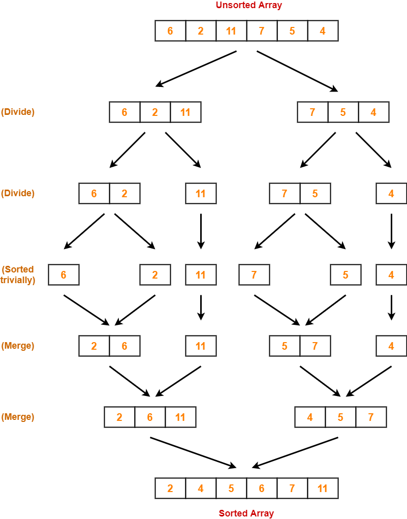
The real work of the algorithm lies in the merge step. This function takes two already-sorted subarrays and combines them into a single, larger sorted array. It does this efficiently by using a two-pointer technique. It places one pointer at the beginning of each subarray and compares the elements. The smaller of the two elements is added to a new temporary array, and that element's pointer is advanced. This process continues until all elements from both subarrays have been moved to the temporary array, which is then copied back.

To see this recursive process in detail, the following video provides an excellent step-by-step trace.

Implementing Merge Sort

Now that you have a strong conceptual model, let's examine the implementation. A typical implementation of Merge Sort consists of two main functions:

• mergeSort(array, low, high): This is the recursive driver function. It finds the middle index of the portion of the array it's responsible for, then calls itself on the left half (low to mid) and the right half (mid+1 to high). After the recursive calls return (meaning the two halves are now sorted), it calls the merge function.
• merge(array, low, mid, high): This helper function performs the merge operation on the two sorted subarrays ([low...mid] and [mid+1...high]) using a temporary array.

The following resource provides clean, modern code for the algorithm in several languages.

Performance Analysis: Why Merge Sort is O(n log n)

One of the most significant advantages of Merge Sort is its consistent and predictable performance. It has a time complexity of O(n log n) in the best, average, and worst cases. Let's break down why.

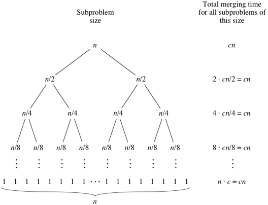
We can analyze the work done by visualizing the recursive calls as a tree.

1. The log n Factor (The Tree's Height): The "Divide" step repeatedly splits the array in half. For an array of size n, you can perform this division log₂ n times before you're left with subarrays of size 1. This means the recursion tree has log n levels of depth.

2. The n Factor (Work per Level): The "Combine" step is the merge operation. At each level of the recursion tree, we are merging a set of subarrays. While the subarrays get smaller as we go down, there are more of them. The crucial insight is that the total number of elements processed across all merges at any single level is always n. Since the merge operation is linear, the total work done at each level is O(n).

By combining these two parts, we get log n levels, each requiring O(n) work, for a total time complexity of O(n log n).

This relationship is formally captured by a recurrence relation.

Space Complexity and Practical Trade-offs

The guaranteed O(n log n) time complexity of Merge Sort does not come for free. Its primary trade-off is its space complexity.

As we saw in the implementation, the merge function requires a temporary array to hold the merged result. The size of this temporary storage is proportional to the number of elements being merged. In the worst case (the final merge of the two halves of the original array), this requires space for n elements. Therefore, the space complexity of Merge Sort is O(n).

This makes Merge Sort an out-of-place algorithm. This is a critical consideration in memory-constrained environments.

Another important characteristic of Merge Sort is that it is a stable sort. This means if two elements have equal values, their original relative order is preserved in the sorted output. This property is valuable in many real-world scenarios, such as when you need to sort data on multiple criteria.

Conclusion

In this lesson, we dissected the Merge Sort algorithm. It serves as a fantastic illustration of the Divide and Conquer paradigm and provides a reliable, efficient method for sorting data.

Here are the essential takeaways:

• Core Idea: Merge Sort works by recursively dividing an array into halves until single-element arrays are reached, then merging them back together in sorted order.
• Time Complexity: It has a consistent time complexity of O(n log n) for all cases (best, average, and worst) because the work is evenly divided at each step.
• Space Complexity: Its main drawback is the need for auxiliary storage, giving it a space complexity of O(n).
• Stability: Merge Sort is a stable sorting algorithm, which can be a crucial feature for certain data processing tasks.

In our next lesson, we will explore another giant of sorting algorithms: Quicksort. We will implement it and then conduct a detailed comparison of its practical trade-offs with Merge Sort. This will highlight a classic engineering decision: choosing between an algorithm with guaranteed performance (Merge Sort) and one that is often faster in practice but has a less favorable worst-case scenario (Quicksort).