PCA for Face Recognition and Visualization

Introduction

In our last lesson, you successfully implemented the Principal Component Analysis algorithm from scratch using Singular Value Decomposition (SVD). This was a crucial step in moving from the theory of PCA—understanding it as the eigendecomposition of the covariance matrix—to its practical, numerically stable implementation.

Today, we put that knowledge into practice with a classic and visually intuitive application of PCA. Our learning outcome is to apply PCA to a high-dimensional dataset of human faces and visualize the principal components.

This project-based lesson will guide you through the "Eigenfaces" method. You will see how a collection of images, each representing a point in a very high-dimensional space, can be analyzed to find its most important features. We will load a real-world dataset, use a professional library (Scikit-learn) to perform PCA, and interpret the results by visualizing the principal components and reconstructing images.

1. The "Eigenface" Concept

Before we start coding, let's establish the core idea. How can an image be treated as a data point for PCA?

An image is a grid of pixels. A grayscale image of size 112x92 pixels can be "flattened" or "unrolled" into a single vector containing $112\times 92=10,304$ pixel values. This vector is a single point in a 10,304-dimensional space. A dataset of 400 such images can be arranged into a data matrix $\mathbf{X}$ of shape (400, 10304).

Applying PCA to this matrix means finding the principal components of this "face space". These components are vectors of length 10,304. When we reshape them back to their original 112x92 image dimensions, they appear as blurry, ghost-like faces. These are the Eigenfaces.

Each eigenface represents a fundamental direction of variance in the dataset—for example, changes in lighting, facial expression, or structural features like nose shape. Any face in the dataset (and even new faces) can be approximated as a weighted sum of these eigenfaces.

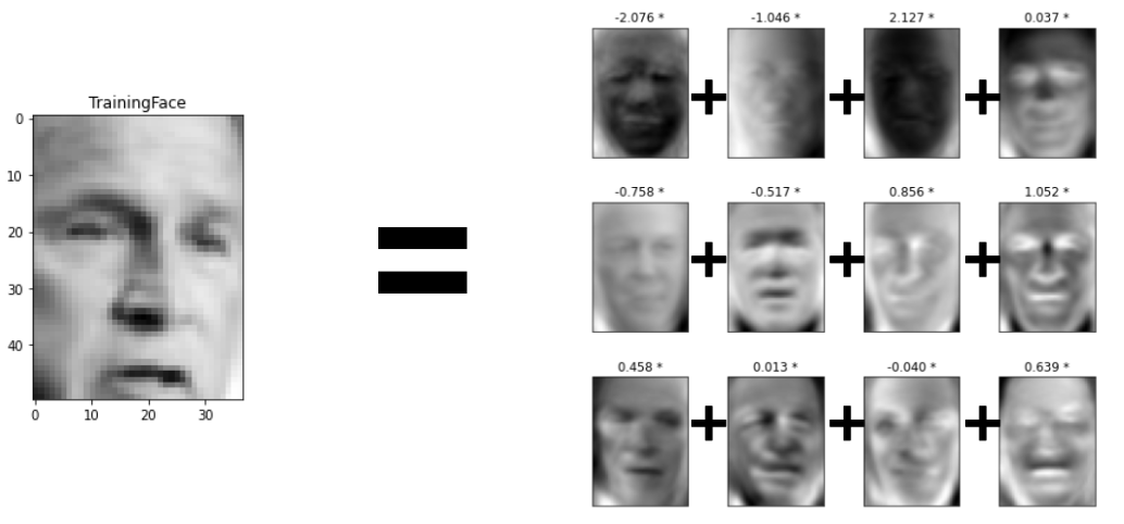
To get a solid grasp of the history and theory behind this method, let's start with a brief reading.

2. Project: Implementing Eigenfaces in Python

Now, let's get our hands dirty. We will work through a complete project using Python. You will need a Python environment with numpy, matplotlib, scikit-learn, and opencv-python installed.

The following reading provides a comprehensive, step-by-step guide to implementing the eigenface method. Your main task for this lesson is to follow this guide, run the code, and ensure you understand the purpose of each step.

3. Analyzing the Results

After completing the guided project, let's dive deeper into some of the key steps and outputs.

Visualizing the Principal Components (Eigenfaces)

The pca.components_ attribute of the fitted Scikit-learn object holds the principal components. For our face data, these are the eigenfaces. The code in the article shows you how to visualize them. They should look something like this:

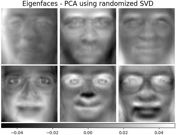
These components form an orthogonal basis for the "face space." The first component is the direction of maximum variance, the second is the orthogonal direction with the next highest variance, and so on.

Choosing the Number of Components

In the project, the number of components (n_components = 50) was chosen somewhat arbitrarily. In a real-world scenario, you would make a more informed decision. The standard method is to plot the cumulative explained variance.

This plot shows how much of the total variance in the original data is captured as we add more principal components.

Now, try generating this plot for the face dataset you just worked with. The code is simple:

import matplotlib.pyplot as plt
import numpy as np



# Assuming 'pca' is the PCA object you fitted in the project

plt.figure(figsize=(10, 7))
plt.plot(np.cumsum(pca.explained_variance_ratio_))
plt.xlabel('Number of Components')
plt.ylabel('Cumulative Explained Variance')
plt.title('Explained Variance by Number of Components')
plt.grid(True)
plt.show()

From your plot, how many components are needed to capture 90% of the variance in the data? This is a much more robust way to select n_components.

Reconstructing Faces from Components

The most powerful way to understand what PCA is doing is to see it in reverse. We can take a low-dimensional representation of a face (its weight vector) and reconstruct the full-dimensional image.

The process is:

1. Transform: Project an original image onto the eigenface basis to get its weight vector.
   weights = pca.transform(image_vector)
2. Inverse Transform: Reconstruct the image from the weights.
   reconstructed_image_vector = pca.inverse_transform(weights)

This is conceptually identical to the image compression example you saw in the last lesson, where a low-rank approximation of the image matrix was created.

Now, let's apply this to our face data. The following code snippet shows how to compare an original image with its reconstruction using 50 components.

# Assuming 'faces' and 'pca' are from your project
# Select an image to test (e.g., the first image of subject 1)
original_image = faces['s1/1.pgm']
original_vector = original_image.flatten().reshape(1, -1)




# Transform to the low-dimensional space
weights = pca.transform(original_vector)




# Inverse transform back to the original space
reconstructed_vector = pca.inverse_transform(weights)
reconstructed_image = reconstructed_vector.reshape(original_image.shape)




# Visualize the comparison
fig, axes = plt.subplots(1, 2, figsize=(8, 4))
axes[0].imshow(original_image, cmap='gray')
axes[0].set_title('Original')
axes[1].imshow(reconstructed_image, cmap='gray')
axes[1].set_title('Reconstructed (50 Components)')
plt.show()

Run this code. The reconstructed image will be slightly blurrier than the original, representing the information lost by discarding the less significant principal components. This visually demonstrates the trade-off between compression and fidelity.

Conclusion

Congratulations on completing this project! You've successfully moved from PCA theory to a significant, practical application.

Key Takeaways:

• High-dimensional data, such as images, can be represented as vectors and analyzed with techniques like PCA.
• The principal components of a face dataset are called Eigenfaces, which form a basis representing the most significant variations in facial appearance.
• Visualizing the cumulative explained variance is a principled method for choosing the number of components to retain.
• PCA allows for dimensionality reduction by transforming data into a lower-dimensional space and reconstruction back to the original space, which provides a powerful way to visualize information loss.

Preview of the Next Lesson

This lesson concludes our deep dive into PCA and marks a transition in the course. You have now mastered a cornerstone of classical machine learning for dimensionality reduction.

In the next and final module, Introduction to Neural Networks, we will explore a different paradigm of learning. We will start from the ground up, deriving the Perceptron algorithm and understanding its limitations, which will motivate the development of Multi-Layer Perceptrons (MLPs) and the powerful backpropagation algorithm.