Perceptron Learning Rule Derivation

1. The Perceptron: A Mathematical Model of a Neuron

The Perceptron was one of the earliest models of a neuron, proposed by Frank Rosenblatt in 1957. It's a binary classifier that makes its decisions based on a linear combination of its inputs.

To get a clear picture of the Perceptron's components, let's watch a brief introductory video.

As the video explained, a Perceptron computes a weighted sum of its inputs, adds a bias, and passes the result through an activation function. For a single training instance with an input vector $\mathbf{x}=[x_1,x_2,...,x_d{]}^T$, a weight vector $\mathbf{w}=[w_1,w_2,...,w_d{]}^T$, and a bias $b$, the process is:

1. Compute the net input ($z$): This is a linear combination.

   $$z={\mathbf{w}}^T\mathbf{x}+b=\sum _{i=1}^d{w}_i{x}_i+b$$

2. Apply an activation function: The original Perceptron uses a Heaviside step function to produce the output $a$. For binary classification with labels {0, 1}:

   $$a=\{\begin{array}{ll}1& \text{if }z\ge 0\\ 0& \text{if }z<0\end{array}$$

The equation $z=0$ defines a hyperplane, which is the decision boundary that separates the input space into two regions. The Perceptron learns by adjusting $\mathbf{w}$ and $b$ to place this boundary correctly.

2. Deriving the Weight Update Rule

The core question is: how does the Perceptron learn the optimal values for $\mathbf{w}$ and $b$? It does so iteratively. It processes one training example at a time and, if it makes a mistake, it adjusts the weights and bias to correct that mistake.

An Intuitive Derivation

Let's think logically about the two possible types of mistakes and how we should respond. We'll denote the learning rate by $\alpha$, a small positive constant that controls the step size.

• Case 1: False Negative. The true label $t=1$, but the Perceptron predicts $a=0$.

  • What happened? This means the net input $z={\mathbf{w}}^T\mathbf{x}+b$ was negative, when it should have been positive.
  • How to fix it? We need to increase $z$. We can achieve this by pushing the weight vector $\mathbf{w}$ "closer" to the input vector $\mathbf{x}$ and increasing the bias $b$.
  • The Update: $${\mathbf{w}}_{\text{new}}={\mathbf{w}}_{\text{old}}+\alpha \mathbf{x}$$ $$b_{\text{new}}=b_{\text{old}}+\alpha$$

• Case 2: False Positive. The true label $t=0$, but the Perceptron predicts $a=1$.

  • What happened? This means the net input $z={\mathbf{w}}^T\mathbf{x}+b$ was non-negative, when it should have been negative.
  • How to fix it? We need to decrease $z$. We can do this by pushing the weight vector $\mathbf{w}$ "away" from the input vector $\mathbf{x}$ and decreasing the bias $b$.
  • The Update: $${\mathbf{w}}_{\text{new}}={\mathbf{w}}_{\text{old}}-\alpha \mathbf{x}$$ $$b_{\text{new}}=b_{\text{old}}-\alpha$$

If the prediction is correct ($t=a$), we make no changes.

Unifying the Rule

We can express these separate rules in a single, elegant equation. Let's define the error for a single sample as $e=t-a$.

• In Case 1 (False Negative): $t=1,a=0⟹e=1$. The update is $\mathbf{w}\leftarrow \mathbf{w}+\alpha (1)\mathbf{x}$.
• In Case 2 (False Positive): $t=0,a=1⟹e=-1$. The update is $\mathbf{w}\leftarrow \mathbf{w}+\alpha (-1)\mathbf{x}$.
• If correct: $t=a⟹e=0$. The update is $\mathbf{w}\leftarrow \mathbf{w}+\alpha (0)\mathbf{x}$, which means no change.

Combining these, we get the Perceptron weight update rule:

And the bias update rule:

This simple rule is the heart of the Perceptron algorithm. The following resource provides a detailed walkthrough of this derivation.

A Formal Derivation using Gradient Descent

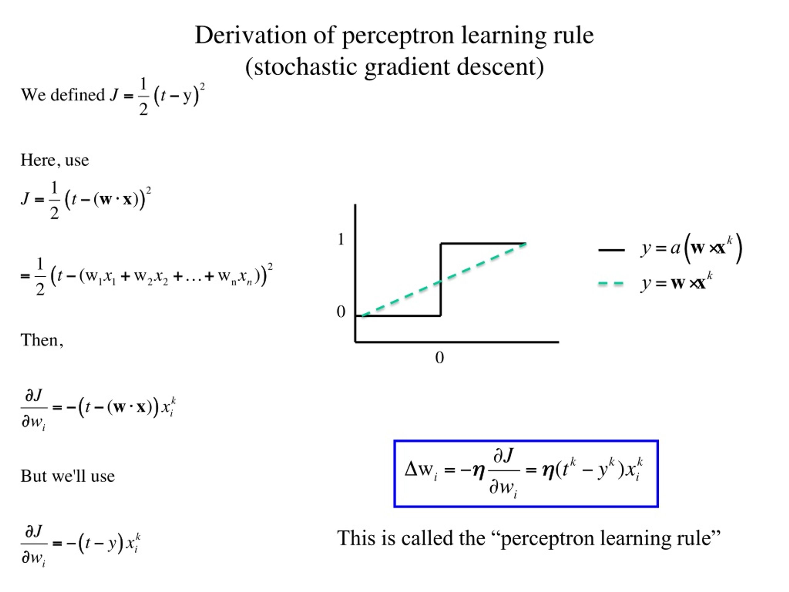
As you appreciate formal proofs, let's derive this rule from a more fundamental optimization perspective. The learning rule can be seen as a form of stochastic gradient descent (SGD). In SGD, we update weights by taking a step in the opposite direction of the gradient of a loss function.

Let's define a loss function for a single training example $(\mathbf{x},t)$. A common choice (though not the only one) is the squared error:

where $f$ is the step activation function.

Because the step function's derivative is zero almost everywhere and infinite at the origin, it's not ideal for gradient descent. However, Rosenblatt's update rule can be formally derived by applying gradient descent to the net input $z={\mathbf{w}}^T\mathbf{x}+b$ before the non-differentiable activation function.

Let's define the loss based on the difference between the target label and the net input, an approach sometimes called the "Perceptron criterion":

This is a simplification, but let's see where it leads. The gradient of this loss with respect to a single weight $w_j$ is:

The approximation comes from the fact that the Perceptron rule uses the final output $a$ instead of the net input. The gradient with respect to the bias is simply $-(t-a)$.

The gradient descent update rule is $\mathbf{w}\leftarrow \mathbf{w}-\alpha {\nabla }_{\mathbf{w}}J$. Applying this gives:

In vector form, this is exactly the Perceptron update rule we derived intuitively.

3. The Algorithm and Its Convergence

Now that we have the update rule, we can state the full algorithm.

The Perceptron Learning Algorithm

1. Initialize the weight vector $\mathbf{w}$ and bias $b$ (e.g., to zeros or small random values).
2. Set a learning rate $\alpha$ (e.g., 0.1) and a number of epochs (passes through the data).
3. For each epoch:
   1. Shuffle the training data.
   2. For each training sample $({\mathbf{x}}_i,t_i)$:
      1. Compute the output $a_i=f({\mathbf{w}}^T{\mathbf{x}}_i+b)$.
      2. Update the weights and bias: $$\mathbf{w}\leftarrow \mathbf{w}+\alpha (t_i-a_i){\mathbf{x}}_i$$ $$b\leftarrow b+\alpha (t_i-a_i)$$

This iterative process of adjusting the decision boundary based on misclassified points has a powerful theoretical guarantee.

Perceptron Convergence Theorem

A remarkable property of this algorithm is that if the training data is linearly separable, the Perceptron learning algorithm is guaranteed to find a solution (i.e., a set of weights and a bias that perfectly classifies all training points) in a finite number of steps.

Let's watch a video that explores the geometric intuition behind the updates and the conditions required for convergence.

The key takeaway is that while the standard definition of linear separability allows points to lie directly on the decision boundary, the Perceptron algorithm's convergence is only guaranteed under the stricter condition that a "margin" or gap exists between the classes.

Conclusion

In this lesson, we have dissected the Perceptron, the foundational model of neural networks. We started with its simple mathematical structure and then, fulfilling the lesson's main goal, derived its learning rule from both intuitive and formal perspectives.

Key Takeaways:

• The Perceptron is a binary linear classifier that computes a weighted sum of inputs and applies a step activation function.
• The Perceptron learning rule, $\mathbf{w}\leftarrow \mathbf{w}+\alpha (t-a)\mathbf{x}$, adjusts the weights and bias only when a misclassification occurs.
• This rule can be derived intuitively by considering how to correct classification errors or formally as a form of stochastic gradient descent.
• The Perceptron Convergence Theorem guarantees that the algorithm will find a separating hyperplane in a finite number of steps, provided the data is linearly separable with a margin.

Preview of the Next Lesson

We've established the Perceptron's power but also hinted at its fundamental limitation: it can only solve problems that are linearly separable. What about problems like the simple XOR logical function, which cannot be solved with a single straight line?

In our next lesson, we will address this limitation by moving from a single Perceptron to a Multi-Layer Perceptron (MLP). You will learn how stacking layers of these simple units allows us to model complex, non-linear decision boundaries and solve a much wider class of problems.