From Perceptrons to MLPs: Overcoming Limitations

1. The Perceptron's Achilles' Heel: The XOR Problem

A single-layer Perceptron works by creating a single linear decision boundary—a line in 2D, a plane in 3D, or a hyperplane in higher dimensions. This works perfectly for problems that are linearly separable, meaning the different classes can be separated by one such hyperplane.

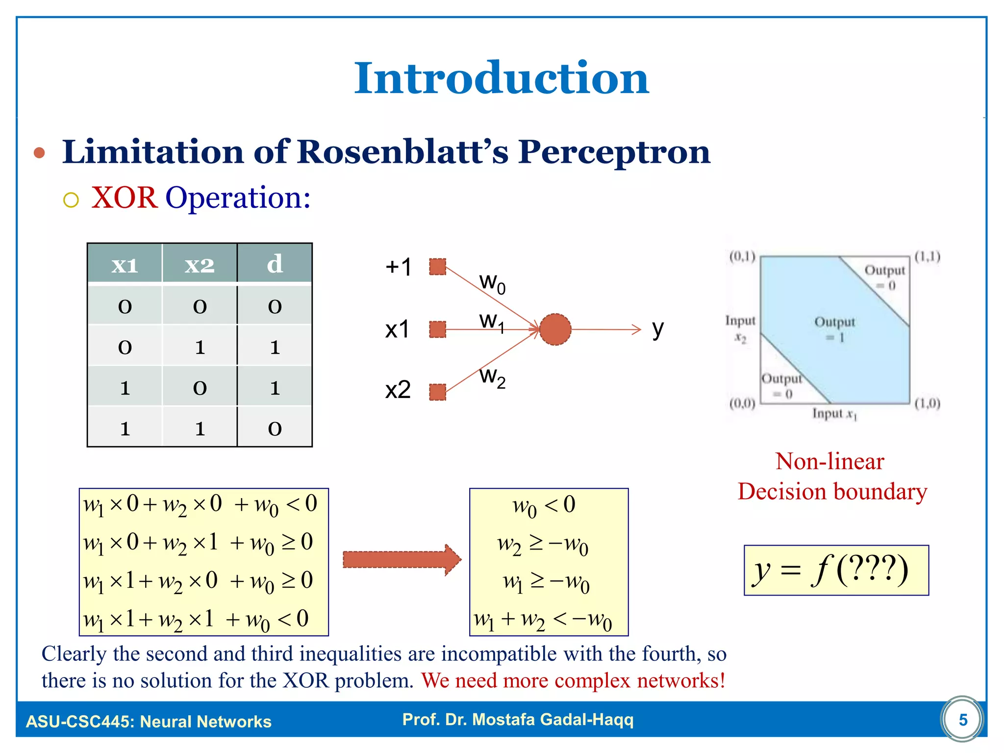
The classic example of a problem that is not linearly separable is the XOR (exclusive OR) function.

To understand precisely why the Perceptron fails here, let's dive into a detailed explanation.

As the reading demonstrates, no single line can separate the (0,1) and (1,0) inputs (which should be class 1) from the (0,0) and (1,1) inputs (which should be class 0). The mathematical proof solidifies this by showing that the constraints imposed by the four XOR data points lead to a logical contradiction.

This inability to handle non-linear relationships was a major criticism of early neural network models and a primary motivation for developing more sophisticated architectures.

2. The Solution: Stacking Layers to Form a Multi-Layer Perceptron (MLP)

If one Perceptron creates one line, what if we could combine multiple lines to create more complex decision boundaries? This is the core idea behind the Multi-Layer Perceptron (MLP).

An MLP consists of:

1. An Input Layer, which receives the raw data features.
2. One or more Hidden Layers, which are not directly connected to the input or output. These are the workhorses of the network.
3. An Output Layer, which produces the final prediction.

A crucial element, which you might recall from our previous lesson, is the non-linear activation function (e.g., the Sigmoid function, ReLU). If we were to only use linear activation functions (or no activation function), stacking multiple layers would be mathematically equivalent to a single layer. The non-linearity is what allows each layer to learn progressively more complex features from the output of the previous layer.

3. How MLPs Create Non-Linear Boundaries

The magic of the MLP lies in what the hidden layer does. Instead of trying to separate the data in the original input space, the hidden layer transforms the input data into a new representation space. In this new space, the problem becomes linearly separable. The output layer is then simply a linear classifier (like a Perceptron) that operates on this transformed, separable data.

Let's watch a video that provides a beautiful visual intuition for this process.

The video shows that the network learns to "un-twist" the complicated data. The hidden layers perform a non-linear mapping $\varphi (\mathbf{x})$ that sends the input data $\mathbf{x}$ into a new feature space where the classes are cleanly separated. The final layer then has the simple job of drawing a line to separate these new, well-behaved clusters.

4. Solving the XOR Problem with an MLP: A Concrete Example

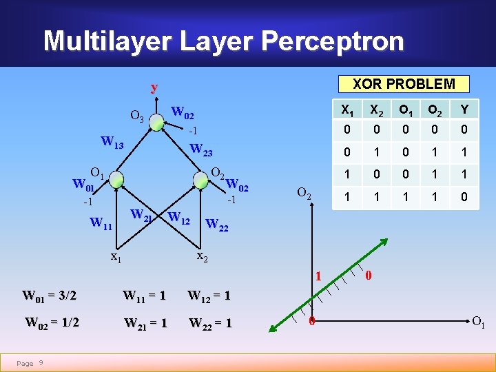
Let's make this tangible by constructing an MLP that solves the XOR problem. We will use a network with 2 input neurons, 2 hidden neurons, and 1 output neuron.

The following video walks through this example in detail, showing the exact weights and calculations needed.

Let's summarize the key insight from the video.
The first hidden neuron, $h_1$, can be trained to learn the OR function. Its decision boundary separates (0,0) from the rest.
The second hidden neuron, $h_2$, can be trained to learn the NAND (NOT AND) function. Its boundary separates (1,1) from the rest.

The hidden layer's output for each input is:

• input(0,0) -> hidden(0,1)
• input(0,1) -> hidden(1,1)
• input(1,0) -> hidden(1,1)
• input(1,1) -> hidden(1,0)

Look at this new representation in the hidden space! The original inputs (0,1) and (1,0) that should be class 1 are now both mapped to (1,1). The original inputs (0,0) and (1,1) that should be class 0 are now mapped to (0,1) and (1,0). In this new 2D space defined by the hidden neurons' activations, the problem is now linearly separable. The output neuron can easily learn an AND function that says "output 1 only if the input from the hidden layer is (1,1)".

Conclusion

In this lesson, we have confronted the fundamental limitation of the Perceptron and introduced its powerful successor, the Multi-Layer Perceptron.

Key Takeaways:

• A single-layer Perceptron can only solve linearly separable problems because its decision boundary is a single hyperplane.
• The XOR problem is the canonical example of a non-linearly separable problem that a Perceptron cannot solve.
• Multi-Layer Perceptrons (MLPs) overcome this limitation by introducing one or more hidden layers with non-linear activation functions.
• The hidden layers learn to transform the input data into a new, higher-dimensional representation where the data becomes linearly separable. The output layer then acts as a simple linear classifier on this transformed data.

Preview of the Next Lesson

We have now manually constructed an MLP with specific weights and biases to solve the XOR problem. This demonstrates that a solution exists. But this raises the most important question: how can a network learn these weights and biases automatically from data?

The intuitive update rule we used for the single Perceptron won't work, because we don't have "correct" labels for the hidden neurons. The next lesson will tackle this challenge head-on as we derive the backpropagation algorithm, the engine that drives the training of almost all modern neural networks. This derivation, which relies heavily on the chain rule from calculus, will be a cornerstone of our course.