Backpropagation: The Chain Rule in Action

Introduction

Welcome to the next lesson in our journey into neural networks. In the previous lesson, we established a crucial point: Multi-Layer Perceptrons (MLPs) can solve non-linearly separable problems like XOR by using hidden layers to transform the data into a space where it becomes linearly separable. We proved a solution can exist by manually constructing a network with specific weights.

However, the true power of neural networks lies in their ability to learn these weights from data automatically. This brings us to the central question: How does the network know how to adjust its internal, hidden weights to reduce the final output error?

This lesson will answer that question by deriving the backpropagation algorithm. This algorithm is the engine that powers the training of most modern neural networks. At its core, backpropagation is a clever and efficient application of the chain rule from calculus to compute the gradient of the cost function with respect to every single weight and bias in the network. Once we have these gradients, we can use gradient descent to iteratively update the parameters and "teach" the network.

Your strong background in mathematics and physics will be a great asset here, as the concepts of propagating sensitivities and applying the chain rule through a multi-stage system are fundamental to this process.

1. Conceptual Framework: Backpropagation as Propagating Error

Before diving into the equations, it's essential to build a strong mental model of what backpropagation does. The goal of training is to minimize a cost function. Using gradient descent, this means we need to calculate how a small change in each weight affects the final cost.

The challenge is that the weights in the early layers of the network influence the cost only indirectly, through all the subsequent layers. Backpropagation provides a way to attribute the final error back to each of these weights, layer by layer, starting from the output and moving backward to the input.

The following video from 3Blue1Brown provides an exceptional visualization of this process.

Backpropagation calculus | Deep Learning Chapter 4

In 'Backpropagation calculus', Grant Sanderson masterfully explains the intuition behind backpropagation, framing it as the application of the chain rule to understand the sensitivity of the cost function to each parameter in the network.

Please watch the video from the beginning to 09:42. Focus on how a small change ('nudge') to a weight propagates through the network to cause a change in the final cost. Pay close attention to how the chain rule is used to break this overall sensitivity down into a product of local sensitivities at each step.

The video beautifully illustrates the core concepts:

The network is a chain of functions, where the output of one layer is the input to the next.
The chain rule allows us to calculate the derivative of the final cost with respect to any parameter by multiplying the local derivatives at each stage of the network.
The gradient calculation for a layer depends on the gradient information from the layer ahead of it. This is the "backward" flow of information.

2. The Mathematical Derivation of Backpropagation

Now, let's formalize the intuition from the video. We will derive the update rules for a simple MLP with one hidden layer. To make this concrete, let's consider the network architecture shown below, with an input layer, a hidden layer, and an output layer.

Neural Network Gradients and Backpropagation Flow — This diagram illustrates the forward and backward passes for a two-layer neural network. We will derive the mathematical expressions for the gradients (∇W1, ∇b1, ∇W2, ∇b2) shown in the backward pass.

We will follow the detailed derivation presented in the article "The Multilayer Perceptron - Theory and Implementation". This resource provides a clear, step-by-step walkthrough that is perfect for understanding the mechanics.

First, let's establish our notation, which will closely follow the article:

Layers: Superscript (L) for the output layer, (L-1) for the hidden layer.
Linear Input: $z^{(l)}$ is the weighted sum of inputs to layer $l$ before activation: $z^{(l)} = a^{(l - 1)} W^{(l)} + b^{(l)}$ .
Activation: $a^{(l)}$ is the output of layer $l$ after the activation function: $a^{(l)} = σ (z^{(l)})$ . The input data is $a^{(0)} = X$ .
Cost Function: We'll use the Mean Squared Error (MSE) for a single example: $E = \frac{1}{2} (a^{(L)} - y)^{2}$ .
Indices: We'll use $j$ for neurons in the output layer, $k$ for neurons in the hidden layer, and $i$ for features in the input layer.

2.1. The Gradient of the Output Layer

We start with the parameters connecting the hidden layer to the output layer: the weights $w_{j k}^{(L)}$ and biases $b_{j}^{(L)}$ . The goal is to find $\frac{\partial E}{\partial w _{j k}^{(L)}}$ .

Using the chain rule, we can decompose this derivative as:

\frac{\partial E}{\partial w _{j k}^{(L)}} = \frac{\partial E}{\partial a _{j}^{(L)}} \cdot \frac{\partial a _{j}^{(L)}}{\partial z _{j}^{(L)}} \cdot \frac{\partial z _{j}^{(L)}}{\partial w _{j k}^{(L)}}

Let's compute each term:

How the error changes with the output activation:
$\frac{\partial E}{\partial a _{j}^{(L)}} = (a_{j}^{(L)} - y_{j})$
How the activation changes with its linear input (derivative of sigmoid):
$\frac{\partial a _{j}^{(L)}}{\partial z _{j}^{(L)}} = σ^{'} (z_{j}^{(L)}) = a_{j}^{(L)} (1 - a_{j}^{(L)})$
How the linear input changes with the weight:
$\frac{\partial z _{j}^{(L)}}{\partial w _{j k}^{(L)}} = a_{k}^{(L - 1)}$

Combining these, we get the gradient for an output layer weight:

\frac{\partial E}{\partial w _{j k}^{(L)}} = (a_{j}^{(L)} - y_{j}) \cdot a_{j}^{(L)} (1 - a_{j}^{(L)}) \cdot a_{k}^{(L - 1)}

It is common to define an "error term" $δ_{j}^{(L)}$ for each output neuron $j$ :

δ_{j}^{(L)} = \frac{\partial E}{\partial z _{j}^{(L)}} = \frac{\partial E}{\partial a _{j}^{(L)}} \cdot \frac{\partial a _{j}^{(L)}}{\partial z _{j}^{(L)}} = (a_{j}^{(L)} - y_{j}) \cdot a_{j}^{(L)} (1 - a_{j}^{(L)})

With this, the gradient is simply:

\frac{\partial E}{\partial w _{j k}^{(L)}} = δ_{j}^{(L)} \cdot a_{k}^{(L - 1)}

2.2. The Gradient of the Hidden Layer

Now for the crucial part: finding the gradient for the hidden layer weights, $\frac{\partial E}{\partial w _{k i}^{(L - 1)}}$ . The chain rule structure is similar:

\frac{\partial E}{\partial w _{k i}^{(L - 1)}} = \frac{\partial E}{\partial a _{k}^{(L - 1)}} \cdot \frac{\partial a _{k}^{(L - 1)}}{\partial z _{k}^{(L - 1)}} \cdot \frac{\partial z _{k}^{(L - 1)}}{\partial w _{k i}^{(L - 1)}}

The last two terms are straightforward derivatives of the activation and linear functions. The key is the first term, $\frac{\partial E}{\partial a _{k}^{(L - 1)}}$ . A hidden neuron's activation $a_{k}^{(L - 1)}$ affects the final error $E$ through every output neuron it is connected to.

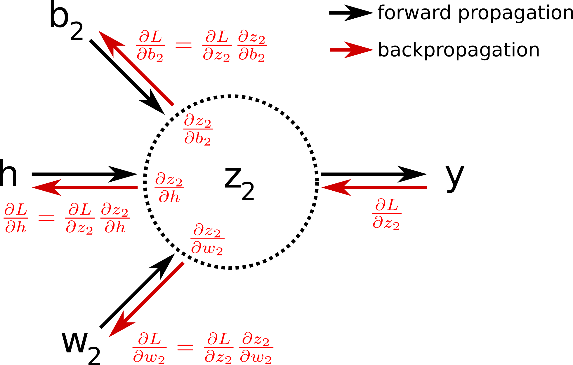
Backpropagation in a Single Neuron — This diagram shows how the error from the output layer is propagated backward. The gradient with respect to a hidden activation 'h' depends on its contribution to the pre-activation 'Z2' of the output neuron, which in turn affects the loss 'L'.

We must sum these influences. The activation $a_{k}^{(L - 1)}$ influences each $z_{j}^{(L)}$ , which in turn influences $E$ . So, we apply the chain rule again:

\frac{\partial E}{\partial a _{k}^{(L - 1)}} = j \sum \frac{\partial E}{\partial z _{j}^{(L)}} \cdot \frac{\partial z _{j}^{(L)}}{\partial a _{k}^{(L - 1)}}

We recognize the first term in the sum as our error term $δ_{j}^{(L)}$ from the output layer. The second term is simply the weight connecting the hidden neuron $k$ to the output neuron $j$ :

\frac{\partial z _{j}^{(L)}}{\partial a _{k}^{(L - 1)}} = w_{j k}^{(L)}

So, we have a way to calculate the error term for the hidden layer, $δ_{k}^{(L - 1)}$ , by using the error terms from the next layer ( $L$ ):

δ_{k}^{(L - 1)} = \frac{\partial E}{\partial z _{k}^{(L - 1)}} = (j \sum δ_{j}^{(L)} \cdot w_{j k}^{(L)}) \cdot a_{k}^{(L - 1)} (1 - a_{k}^{(L - 1)})

This equation is the heart of backpropagation. It shows how the error is propagated backward: the error at a hidden neuron is a weighted sum of the errors of the neurons it connects to in the next layer.

Finally, we can compute the gradient for the hidden layer weight:

\frac{\partial E}{\partial w _{k i}^{(L - 1)}} = δ_{k}^{(L - 1)} \cdot a_{i}^{(L - 2)}

where $a_{i}^{(L - 2)}$ is simply the $i$ -th input feature, $x_{i}$ .

For a thorough, line-by-line derivation of these equations, including the gradients for the bias terms, please study the following resource.

The Multilayer Perceptron - Theory and Implementation of the Backpropagation Algorithm

The article 'The Multilayer Perceptron - Theory and Implementation' by Pablo Insente provides a very clear mathematical formalization of backpropagation. We have just outlined the core logic; this article will fill in all the details.

Please read the section 'Backpropagation algorithm'. Start from the introduction of the algorithm and follow the derivations closely. First, trace the logic for the 'single unit multilayer perceptron' to solidify the concept, then see how it expands to the 'multiple unit' case with the extra indices and summations. We will discuss the code implementation next.

3. From Calculus to Code: A Modular Perspective

The equations we derived can be implemented directly, but modern deep learning libraries think about backpropagation in a more modular way. Each layer in a network can be seen as an object with two primary methods:

forward(input): Takes an input, performs its computation (e.g., matrix multiplication and activation), and returns an output.
backward(output_gradient): Takes the gradient of the final loss with respect to the layer's output ( $\frac{\partial E}{\partial a ^{(l)}}$ ) and calculates two things:
- The gradient of the loss with respect to the layer's internal parameters ( $\frac{\partial E}{\partial W ^{(l)}}$ ).
- The gradient of the loss with respect to the layer's input ( $\frac{\partial E}{\partial a ^{(l - 1)}}$ ), which it then returns to be passed to the previous layer.

This elegant design allows us to stack any number of layers, and the backpropagation process just works, chaining the gradients backward automatically. The following video explains this programming perspective very well, deriving the gradients using matrix notation, which is how they are computed in practice.

Neural Network from Scratch | Mathematics & Python Code

The video 'Neural Network from Scratch | Mathematics & Python Code' explains the modular implementation of backpropagation, showing how each layer is responsible for its own forward and backward pass.

Watch the following segments: (02:40 - 06:36): This explains the core concept of a layer's 'backward' method passing gradients to the previous layer. (10:35 - 18:22): This provides the detailed mathematical derivation for the gradients of a dense layer using matrix notation. Compare these matrix equations to the element-wise equations we derived earlier. (20:34 - 22:01) and (23:27 - 25:57): These briefly cover the activation layer and the initial error derivative from the loss function, completing the chain.

As you saw, the mathematical derivation, especially when vectorized with matrix operations, translates directly into code. The implementation in the fit function of the "The Multilayer Perceptron" article (LINK) that you read earlier is a perfect, practical example of this.

Conclusion

In this lesson, we have demystified the backpropagation algorithm, revealing it to be a systematic and efficient application of the chain rule for computing the gradients needed for training a neural network.

Key Takeaways:

Backpropagation computes the gradient of the cost function with respect to each weight and bias in the network.
It works by propagating an "error signal" ( $δ$ ) backward from the output layer to the input layer.
The error signal for a given layer ( $δ^{(l)}$ ) is calculated using the error signal from the next layer ( $δ^{(l + 1)}$ ) and the weights connecting them.
This process is a recursive application of the chain rule from calculus.
The computed gradients are then used in an optimization algorithm like gradient descent to update the network's parameters.

Optional Further Study

For those who want to delve even deeper into the mathematics, the provided PDF on matrix calculus offers a more formal treatment. Question 8 in the document is a great self-test that asks you to derive the chain rule for a two-hidden-layer network, which is a direct application of what we've learned.

Matrix Calculus for 10-301/601

For a rigorous treatment of the chain rule for vector and matrix operations, this document provides the formal background.

Skim Section 2.2, 'Chain Rule', to see the formal generalization to vectors. Then, try to solve Question 8 in Section 2. The provided solutions in Section 4.2 will help you check your work.

Preview of the Next Lesson

We have now seen that MLPs can represent non-linear functions and that backpropagation allows them to learn these functions from data. But just how powerful are they? What is the theoretical limit to the kinds of functions an MLP can learn? The next lesson will explore the remarkable Universal Approximation Theorem, which states that a simple MLP with a single hidden layer can, in principle, approximate any continuous function to an arbitrary degree of accuracy.

Recommended resources