The Universal Approximation Theorem

1. What Does "Universal" Mean?

The term "universal" suggests that neural networks can compute, in principle, any function. Before we dive into the formal statement, it's important to clarify this powerful claim with two important caveats.

To begin, let's start with a resource that provides a clear, high-level introduction to the concept of universality and its limitations.

As you've just read, the two critical caveats are:

1. Approximation, not exact computation: The theorem guarantees that a neural network can get arbitrarily close to a target function. It does not mean it can represent it exactly. The quality of the approximation can be improved by increasing the network's size (i.e., the number of neurons).
2. Continuity is key: The class of functions that can be approximated are continuous functions. A network composed of continuous activation functions will itself be a continuous function of its inputs, so it cannot perfectly replicate sharp jumps or discontinuities.

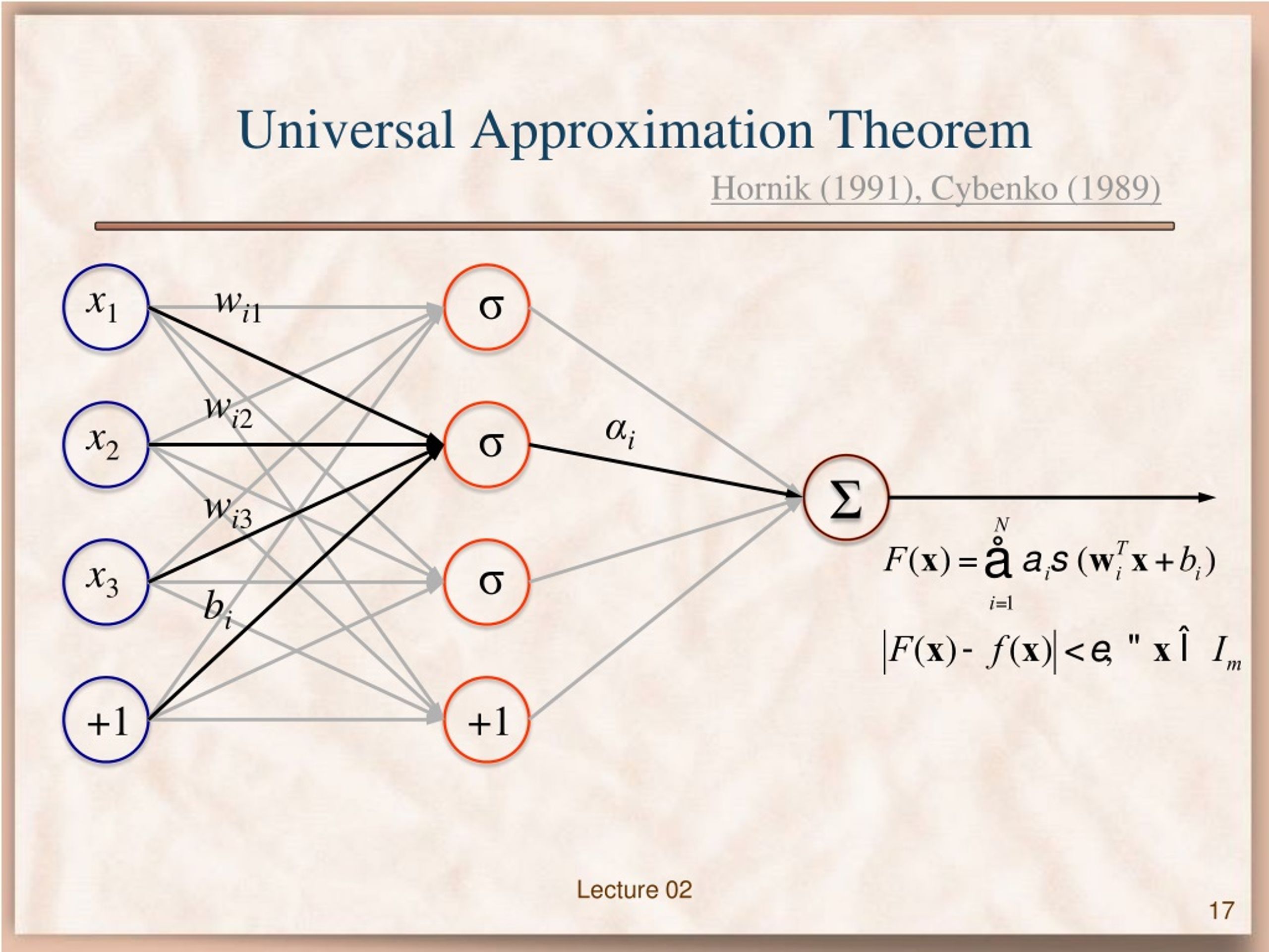
Visually, the theorem states that for a given continuous function f(x), we can construct a neural network F(x) that traces its shape as closely as we desire.

2. The Universal Approximation Theorem: A Formal Look

The theorem can be stated as follows:

A feedforward network with a single hidden layer containing a finite number of neurons can approximate continuous functions on compact subsets of ${\mathbb{R}}^n$, under mild assumptions on the activation function (specifically, that it is not a polynomial). The approximation can be made arbitrarily close to the target function.

Let's break this down:

• Single Hidden Layer: The result is surprisingly strong. We don't need a complex, deep architecture to achieve universality.
• Finite Neurons: While the number of neurons needed might be very large, it is finite.
• Non-Polynomial Activation: This condition is crucial. A network composed of layers of polynomial activations can only ever compute a polynomial of a fixed maximum degree, and thus cannot approximate general non-polynomial functions.

The following image provides a concise visual and mathematical summary of the theorem.

3. A Constructive Proof and Its Intuition

While the formal proofs of the UAT can be quite abstract (often leveraging tools from functional analysis like the Stone-Weierstrass theorem), we can build a strong intuition through a more constructive approach.

3.1. From Building Blocks to Arbitrary Functions

The core idea is to show that a neural network can create simple "building block" shapes, which can then be combined to construct any complex function.

• 1D Case: Creating a "Bump"
  A single neuron with a sigmoidal activation function, $\sigma (wx+b)$, creates a soft "step". By combining two such neurons with opposite weights, we can create a "bump" function. We can control the bump's position (with the bias b), width (with the weight w), and height (with the weights in the output layer). By summing many of these bumps of varying heights, widths, and positions, we can approximate any 1D continuous function, much like a Riemann sum approximates an integral.

• Higher Dimensions: Stacking "Cylinders"
  This idea extends to higher dimensions. In 2D, we can create a smooth "cylinder" function that is high over a small circular region and zero everywhere else. By adding together many such cylinders of different heights and at different locations, we can approximate any 2D surface.

The following video segment provides an excellent visual demonstration of this concept.

3.2 A More Mathematical Construction

For a more rigorous, yet still intuitive, proof sketch, we can see how a network can build up complexity from simple components. This approach will likely resonate with your mathematical background.

This line of reasoning is elegant because it connects the capabilities of neural networks directly to fundamental results in approximation theory.

4. The Power of Depth: A Crucial Implication of the UAT

The UAT guarantees that a single hidden layer is sufficient for universal approximation, but it makes no claim about efficiency. A shallow network might require an astronomical number of neurons to approximate a complex function. This is where deep learning finds its theoretical justification.

Deep networks can be exponentially more efficient at representing certain functions than shallow ones.

This means that for a given level of approximation accuracy, a deep network can often achieve it with far fewer total neurons than a shallow network.

Let's explore this critical trade-off between width and depth.

As the video explained, for functions with a hierarchical or compositional structure (like the parity function), a deep architecture naturally mirrors this structure, leading to a much more compact representation. A shallow network, forced to learn everything in one step, may suffer from the "curse of dimensionality," requiring a number of neurons that grows exponentially with the number of inputs.

5. Practical Consequences and Final Nuances

The UAT is an existence theorem—it tells us a network exists, but it doesn't tell us how to find it. The process of finding the right weights is what we do during training (e.g., via backpropagation and gradient descent), which is a difficult non-convex optimization problem.

Furthermore, the theorem's power depends on the network having sufficient "capacity." A critical insight is that each layer must be wide enough to pass on the necessary information to the next.

Conclusion

This lesson marks the final topic in our course on the foundations of data science. We've journeyed from the basics of probability and statistics, through classical estimation theory and hypothesis testing, to the sophisticated worlds of linear regression, clustering, and finally, neural networks.

The Universal Approximation Theorem serves as a powerful capstone to this journey. It provides the theoretical assurance that the models we are building have the potential to capture the complex, non-linear relationships hidden within data.

Key Takeaways:

• Universal Approximation: A neural network with a single hidden layer and a non-polynomial activation function can approximate any continuous function to arbitrary precision.
• Existence, Not Discovery: The theorem guarantees that a suitable network exists, but it doesn't guarantee that our training algorithms can find it.
• The Advantage of Depth: While a shallow network is theoretically sufficient, a deep network is often exponentially more efficient, requiring far fewer neurons to represent complex, hierarchical functions. This is a core justification for the "deep learning" paradigm.
• Capacity Matters: For a network to be a universal approximator in practice, each layer must be sufficiently wide to avoid creating an information bottleneck.

You now possess a robust framework for understanding not just how data science models work, but also their theoretical capabilities and limitations. The next logical step, as outlined in the course syllabus, is to apply these concepts in a hands-on project, where you will tackle a real-world problem from start to finish. This will be your opportunity to integrate everything you've learned.