Neural Networks for Digit Classification

1. The Problem: Handwritten Digit Classification

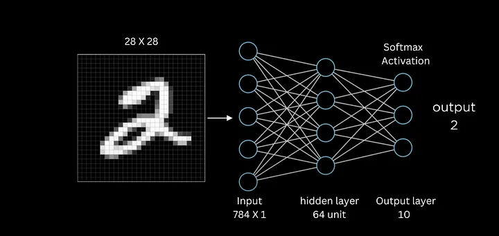
Our goal is to build a model that can look at a small image of a handwritten digit and correctly identify which number it is (from 0 to 9). This is a multiclass classification problem. We will use the MNIST dataset, which contains thousands of 28x28 pixel grayscale images of handwritten digits.

To a computer, a 28x28 pixel image is just a matrix of numbers. To feed this into a standard MLP, we first need to "flatten" this 2D matrix into a 1D vector.

• A 28x28 image has $28\times 28=784$ pixels.
• Each pixel value (from 0 for black to 255 for white) will become a single feature.
• Therefore, our input layer will have 784 neurons.
• Since there are 10 possible digits (0-9), our output layer will have 10 neurons, each corresponding to the probability of the image being a particular digit.

The following video provides an excellent conceptual overview of this setup.

2. A Look Under the Hood: From Math to Code

Before we use a high-level library like Scikit-learn, it's incredibly valuable to see how the concepts we've learned—forward propagation, backpropagation, and gradient descent—are implemented directly in code. This connects the mathematical theory to the practical reality of what the computer is doing.

The following video provides a complete, from-scratch implementation of a neural network for MNIST classification using only Python and NumPy. Watching it will give you a concrete understanding of the algorithms that Scikit-learn abstracts away for us.

Understanding this process is what separates a proficient user from an expert. When a model fails to train, knowing what's happening "under the hood" is essential for debugging.

3. Project: Building with Scikit-learn

Now, let's build our classifier using the MLPClassifier from Scikit-learn. This part is a hands-on guide. I recommend you open a Jupyter notebook or Python script and follow along.

For a detailed reference on the steps we're about to take, the "Introduction to Machine Learning with Scikit Learn" tutorial is a great resource. We will be following a similar workflow.

Step 1: Setup and Data Loading

First, we import the necessary libraries and load the MNIST dataset. fetch_openml is a convenient function for downloading popular datasets.

import numpy as np
import matplotlib.pyplot as plt
import seaborn as sns
from sklearn.datasets import fetch_openml
from sklearn.model_selection import train_test_split
from sklearn.neural_network import MLPClassifier
from sklearn.metrics import accuracy_score, confusion_matrix




# Load data from https://www.openml.org/d/554
X, y = fetch_openml("mnist_784", version=1, return_X_y=True, as_frame=False)

print(f"Data shape: {X.shape}")
print(f"Labels shape: {y.shape}")

You should see that X has a shape of (70000, 784), meaning 70,000 images, each with 784 pixels. y has a shape of (70000,), containing the label for each image.

Step 2: Data Preprocessing

Neural networks train most effectively when input features are on a similar scale. The pixel values in our dataset range from 0 to 255. We will scale them to a range of 0 to 1 by dividing by 255.

We also need to split our data into a training set (for the model to learn from) and a test set (to evaluate its performance on unseen data).

# Scale the pixel values to the [0, 1] range
X_scaled = X / 255.0




# Split data into training and testing sets
X_train, X_test, y_train, y_test = train_test_split(
    X_scaled, y, test_size=0.2, random_state=42, stratify=y
)

print(f"Training data shape: {X_train.shape}")
print(f"Test data shape: {X_test.shape}")

Step 3: Model Definition and Training

Now we define our MLPClassifier. We'll start with a simple architecture: one hidden layer with 50 neurons.

• hidden_layer_sizes=(50,): A tuple where each element is the number of neurons in a hidden layer. (50,) means one hidden layer with 50 neurons. (100, 50) would mean two hidden layers.
• max_iter=50: The number of epochs, or passes over the training data.
• random_state=42: Ensures our results are reproducible.
• verbose=True: Prints progress during training.

Then, we train the model using the .fit() method.

# Initialize the MLPClassifier
mlp = MLPClassifier(
    hidden_layer_sizes=(50,),
    max_iter=50,
    random_state=42,
    verbose=True
)




# Train the model
print("Training the MLPClassifier...")
mlp.fit(X_train, y_train)
print("Training complete.")

You will see the training loss decrease with each iteration, indicating that the model is learning.

Step 4: Model Evaluation

How well did our model learn? We first check its accuracy on both the training data and the unseen test data.

# Evaluate the model
train_accuracy = mlp.score(X_train, y_train)
test_accuracy = mlp.score(X_test, y_test)

print(f"\nTraining set accuracy: {train_accuracy:.4f}")
print(f"Test set accuracy: {test_accuracy:.4f}")

You should see a test accuracy of around 96-97%, which is quite good for a simple model!

Accuracy gives us a single number, but a confusion matrix gives us more insight into what kind of errors the model is making. The matrix shows the true labels versus the predicted labels.

# Make predictions on the test set
y_pred = mlp.predict(X_test)




# Generate the confusion matrix
cm = confusion_matrix(y_test, y_pred)




# Plot the confusion matrix
plt.figure(figsize=(10, 8))
sns.heatmap(cm, annot=True, fmt="d", cmap="Blues")
plt.title("Confusion Matrix")
plt.xlabel("Predicted Label")
plt.ylabel("True Label")
plt.show()

The diagonal elements show the number of correct predictions for each digit. Off-diagonal elements show misclassifications. For example, a non-zero value in the cell for row "7" and column "9" means the model incorrectly predicted a "7" as a "9".

4. Self-Test: Hyperparameter Tuning

You have successfully built and evaluated a neural network. Now it's your turn to be the researcher. The performance of a neural network is highly dependent on its architecture and training parameters, known as hyperparameters.

Your task is to experiment with different hyperparameter values to see if you can improve the test accuracy. Try modifying the MLPClassifier with the following:

1. Network Architecture: Change the hidden_layer_sizes.
   • Try a wider single layer: hidden_layer_sizes=(100,)
   • Try a deeper network: hidden_layer_sizes=(100, 50)
2. Learning Rate: The learning_rate_init parameter controls the step size of gradient descent. The default is 0.001.
   • Try a larger rate: learning_rate_init=0.01
   • What happens if the rate is too large, e.g., learning_rate_init=0.5?
3. Regularization: The alpha parameter adds L2 regularization to prevent overfitting. The default is 0.0001.
   • Try increasing it to alpha=0.01. Does this help or hurt performance?

For each change, re-train the model and observe the effect on the test accuracy and training time. This process of experimentation is central to applied machine learning.

Conclusion

Congratulations on completing the final lesson and the capstone project for DS215!

In this lesson, you have tied together all the major themes of the course. You took a raw dataset, preprocessed it, built a sophisticated model (a neural network), trained it, and evaluated its performance using both quantitative metrics and qualitative tools like the confusion matrix. You saw how a high-level library like Scikit-learn makes complex algorithms accessible, but you also peered "under the hood" to understand the mathematical machinery at work.

Key Takeaways from the Project:

• The ML Workflow: The process of data preparation, model training, and evaluation is a standard workflow for nearly all supervised learning tasks.
• Preprocessing is Crucial: Simple steps like scaling your data can have a huge impact on model performance.
• Evaluation is Nuanced: A single accuracy score is useful, but tools like the confusion matrix provide deeper insights into a model's strengths and weaknesses.
• Hyperparameters Matter: The design choices you make (like network architecture and learning rate) are critical for success.

This project marks the end of our journey through the "Introduction to Data Science." We started with the language of uncertainty—probability—and built upon it to understand statistical inference, estimation, and hypothesis testing. We then used that foundation to explore core machine learning models, from the simplicity of linear regression to the powerful, non-linear world of neural networks.

You have demonstrated great initiative and intellectual curiosity in pursuing this self-study curriculum. The skills and theoretical understanding you have developed are the bedrock of the field and will serve you well as you continue to explore more advanced topics in data science.