PCA with NumPy's SVD

1. Why SVD? A More Stable Path to PCA

From our last lesson, the PCA algorithm is:

1. Mean-center the data matrix $\mathbf{X}$.
2. Compute the covariance matrix $\mathbf{S}\propto {\mathbf{X}}^T\mathbf{X}$.
3. Find the eigenvectors of $\mathbf{S}$.

While correct, step 2—explicitly forming the matrix ${\mathbf{X}}^T\mathbf{X}$—can sometimes lead to a loss of numerical precision. Singular Value Decomposition offers a way to find the same principal components by operating directly on the data matrix $\mathbf{X}$, which is generally more numerically stable.

SVD is a fundamental matrix factorization that states any $n\times p$ matrix $\mathbf{X}$ can be decomposed as:

where:

• $\mathbf{U}$ is an $n\times n$ orthogonal matrix (left singular vectors).
• $\mathbf{\Sigma }$ is an $n\times p$ rectangular diagonal matrix of singular values.
• $\mathbf{V}$ is a $p\times p$ orthogonal matrix (right singular vectors), so ${\mathbf{V}}^T$ is its transpose.

The key question is: how do these new matrices $\mathbf{U}$, $\mathbf{\Sigma }$, and $\mathbf{V}$ relate to the principal components we're looking for?

The following video provides an excellent and concise explanation of this relationship.

2. The Algebraic Connection

As the video demonstrated, the connection is beautifully direct. Let's formalize it. Suppose our data matrix $\mathbf{X}$ is already mean-centered.

The covariance matrix $\mathbf{S}$ is proportional to ${\mathbf{X}}^T\mathbf{X}$. Let's substitute the SVD of $\mathbf{X}$ into this expression:

Since $\mathbf{U}$ is an orthogonal matrix, ${\mathbf{U}}^T\mathbf{U}=\mathbf{I}$ (the identity matrix). This simplifies the equation to:

Now, let's compare this with the eigendecomposition of the covariance matrix $\mathbf{S}\propto {\mathbf{X}}^T\mathbf{X}$, which we know is $\mathbf{S}=\mathbf{P\Lambda }{\mathbf{P}}^T$, where $\mathbf{P}$ is the matrix of eigenvectors and $\mathbf{\Lambda }$ is the diagonal matrix of eigenvalues.

By direct comparison, we see that:

1. The columns of $\mathbf{V}$ (the right singular vectors of $\mathbf{X}$) are the same as the columns of $\mathbf{P}$ (the eigenvectors of ${\mathbf{X}}^T\mathbf{X}$). Therefore, the right singular vectors are the principal components!
2. The diagonal matrix of squared singular values, ${\mathbf{\Sigma }}^T\mathbf{\Sigma }$, is the same as the diagonal matrix of eigenvalues $\mathbf{\Lambda }$ (up to the scaling factor $n-1$). That is, ${\lambda }_i\propto {\sigma }_i^2$.

Furthermore, the projected data points (the principal component scores), which we found were $\mathbf{Z}=\mathbf{XV}$, can also be expressed using SVD:

This gives us a very elegant and efficient way to compute both the principal directions and the transformed data.

The following reading provides a fantastic summary of this relationship, including a Python code snippet that we will build upon.

3. Implementing PCA with SVD

Now we have a new recipe for PCA that avoids computing the covariance matrix:

1. Organize Data: Arrange your data into an $n\times p$ matrix $\mathbf{X}$.
2. Mean-Center: For each feature, subtract its mean.
3. Compute SVD: Perform SVD on the centered matrix ${\mathbf{X}}_{centered}$ to get $\mathbf{U}$, $\mathbf{\Sigma }$, and ${\mathbf{V}}^T$.
4. Identify Principal Components: The principal components are the columns of $\mathbf{V}$, which are the rows of ${\mathbf{V}}^T$.
5. Transform Data: The new coordinates are the columns of $\mathbf{U\Sigma }$.

Let's translate this into Python code.

Your Task: Build a PCA Class from Scratch

Your goal is to implement a simple Python class, MyPCA, that performs PCA using numpy.linalg.svd. This task is inspired by the common structure of Scikit-learn models and will test your ability to translate the SVD-based algorithm into working code.

Here is a skeleton for your class. Your job is to fill in the fit and transform methods.

import numpy as np

class MyPCA:
    def __init__(self, n_components):
        """
        Initialize the PCA transformer.
        :param n_components: The number of principal components to keep.
        """
        self.n_components = n_components
        self.components = None
        self.mean = None

    def fit(self, X):
        """
        Fit the model with X.
        :param X: A numpy array of shape (n_samples, n_features).
        """



        # 1. Mean center the data
        #    - Calculate the mean of X along the sample axis.
        #    - Store it in self.mean.
        #    - Subtract the mean from X.
        



        # --- YOUR CODE HERE ---
        self.mean = # ...
        X_centered = # ...



        # ----------------------




        # 2. Perform SVD
        #    - Use np.linalg.svd on the centered data.
        #    - Remember that np.linalg.svd returns U, s, and V_t (V transpose).
        #    - Set full_matrices=False for efficiency, it gives the "thin" SVD.
        



        # --- YOUR CODE HERE ---
        U, s, Vt = # ...



        # ----------------------




        # 3. Store the principal components
        #    - The principal components are the first `n_components` rows of Vt.
        #    - Store them in self.components.
        



        # --- YOUR CODE HERE ---
        self.components = # ...



        # ----------------------


    def transform(self, X):
        """
        Apply dimensionality reduction to X.
        :param X: A numpy array of shape (n_samples, n_features).
        :return: The transformed data, a numpy array of shape (n_samples, n_components).
        """



        # 1. Mean center the data using the mean calculated in `fit`.
        



        # --- YOUR CODE HERE ---
        X_centered = # ...



        # ----------------------


```grasp
{
  "type": "exercise",
  "id": "52198123-9f4f-4def-a37d-05147522bed5"
}

    # 2. Project the data onto the principal components.
    #    - This is a dot product between the centered data and the components.
    #    - Be mindful of the shape of self.components. You may need to transpose it.
    



    # --- YOUR CODE HERE ---
    X_projected = # ...
    return X_projected



    # ----------------------

Take about 20-25 minutes to complete this implementation. Don't worry about getting it perfect; the goal is to work through the logic.

<details>
<summary>Hint</summary>
*   For the dot product in `transform`, if `self.components` has shape `(n_components, n_features)`, the projection is `X_centered @ self.components.T`.
*   The result of `np.linalg.svd` is already sorted by the importance of the singular values, so you can just take the first `n_components` rows from `Vt`.
</details>




### 4. Verifying the Implementation

Once you have attempted the implementation, let's study a complete, step-by-step example that also verifies the correctness of the SVD approach against the eigendecomposition method.

```grasp
{
  "type": "reading",
  "title": "PCA-SVD: Singular Value Decomposition with Python Step-by-Step",
  "id": "[LINK](https://github.com/christianversloot/machine-learning-articles/blob/main/introducing-pca-with-python-and-scikit-learn-for-machine-learning.md)",
  "url": "https://github.com/christianversloot/machine-learning-articles/blob/main/introducing-pca-with-python-and-scikit-learn-for-machine-learning.md",
  "relevant_section_indices": [
    1
  ],
  "par_intro": "This article, 'PCA-SVD: Singular Value Decomposition with Python Step-by-Step', provides a clean, native Python implementation that mirrors the task you just undertook.",
  "par_directions": "Please read the section 'PCA-SVD: Singular Value Decomposition with Python Step-by-Step'. Compare its logic with your own implementation. Pay close attention to how it performs SVD on the transposed data matrix and builds the projection matrix from the result (`vh`).",
  "estimated_time": "10 minutes"
}

The code in the LINK StackExchange answer provides an even more rigorous validation by using assert statements to numerically prove the equivalence of the two methods.

Here is the completed MyPCA class based on these principles:

import numpy as np

class MyPCA:
    def __init__(self, n_components):
        self.n_components = n_components
        self.components = None
        self.mean = None

    def fit(self, X):



        # 1. Mean center the data
        self.mean = np.mean(X, axis=0)
        X_centered = X - self.mean




        # 2. Perform SVD
        # Note: We work with features as columns, so we don't transpose X.
        U, s, Vt = np.linalg.svd(X_centered, full_matrices=False)




        # 3. Store the principal components
        # The principal components are the rows of Vt.
        self.components = Vt[:self.n_components]

    def transform(self, X):



        # 1. Mean center the data
        X_centered = X - self.mean




        # 2. Project the data
        # X_centered is (n_samples, n_features)
        # self.components is (n_components, n_features)
        # We need to dot X_centered with the transpose of self.components
        X_projected = X_centered @ self.components.T
        return X_projected




# Example Usage:
from sklearn.datasets import load_iris




# Load data
iris = load_iris()
X = iris.data




# Instantiate and use our PCA
pca = MyPCA(n_components=2)
pca.fit(X)
X_transformed = pca.transform(X)

print("Shape of original data:", X.shape)
print("Shape of transformed data:", X_transformed.shape)




# Compare with Scikit-learn
from sklearn.decomposition import PCA as SklearnPCA
from sklearn.preprocessing import StandardScaler




# Scikit-learn's PCA often assumes standardized data
scaler = StandardScaler()
X_scaled = scaler.fit_transform(X)

sklearn_pca = SklearnPCA(n_components=2)
X_sklearn_transformed = sklearn_pca.fit_transform(X_scaled)




# Our implementation on scaled data
my_pca_scaled = MyPCA(n_components=2)
my_pca_scaled.fit(X_scaled)
X_my_transformed_scaled = my_pca_scaled.transform(X_scaled)




# The results should be very close (potentially with a sign flip)
print("\nOur PCA result on scaled data (first 5 rows):\n", X_my_transformed_scaled[:5])
print("\nScikit-learn PCA result (first 5 rows):\n", X_sklearn_transformed[:5])

Conclusion

Congratulations! You have successfully built a working PCA implementation from scratch. This exercise solidifies the deep connection between a core machine learning technique and a fundamental theorem of linear algebra.

Key Takeaways:

• PCA can be performed by applying Singular Value Decomposition directly to the mean-centered data matrix $\mathbf{X}$.
• This approach is numerically more stable than forming the covariance matrix ${\mathbf{X}}^T\mathbf{X}$.
• The right singular vectors (columns of $\mathbf{V}$, or rows of ${\mathbf{V}}^T$) are the principal components.
• The transformed data (principal component scores) can be found by calculating ${\mathbf{X}}_{centered}\mathbf{V}$ or, equivalently, $\mathbf{U\Sigma }$.

Preview of the Next Lesson

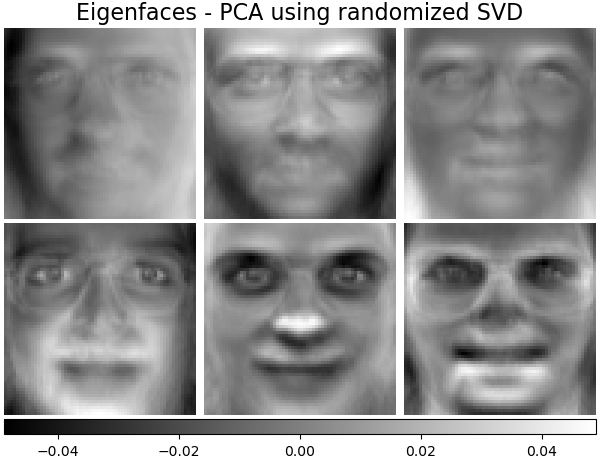
Now that you have built and understood the PCA algorithm, it's time to apply it. In our next lesson, we will undertake a project: applying PCA to a high-dimensional dataset of human faces. We will use our implementation to reduce the dimensionality and visualize the principal components, which in this context are famously known as "Eigenfaces".