Simulating CLT & Law of Large Numbers in Python

Introduction

Welcome to your final lesson in the "Asymptotic Theory and Simulation" module. In our previous lessons, we've built a solid theoretical understanding of two of the most important theorems in probability: the Law of Large Numbers (LLN) and the Central Limit Theorem (CLT). You've derived the Weak Law of Large Numbers from Chebyshev's inequality and outlined the proof of the CLT using characteristic functions.

Today, we transition from theory to practice. This lesson is a hands-on project where you will develop Python simulations to visually demonstrate both the Law of Large Numbers and the Central Limit Theorem. The goal is to solidify your intuition for these theorems, see them in action, and write the code that makes these abstract concepts tangible. For an engineer, simulation is a powerful tool for verifying theoretical models, and today we'll apply that same mindset to these foundational statistical principles.

Project Setup

For this project, you will need a Python environment with the following libraries installed: NumPy, Matplotlib, and SciPy. These are the standard tools for numerical and scientific computing in Python. You will be writing scripts to generate random data, compute statistics, and create visualizations.

Part 1: Simulating the Law of Large Numbers

The Law of Large Numbers tells us that as we increase our sample size, the sample mean $X ˉ_{n}$ gets closer and closer to the true population mean $μ$ . Let's build a simulation to observe this convergence.

A classic and intuitive example is rolling a die. The outcome of a single roll is a random variable from a discrete uniform distribution over ${1, 2, 3, 4, 5, 6}$ . The true population mean, or expected value, is:
$μ = E [X] = \sum_{i = 1}^{6} i \cdot P (X = i) = (1 + 2 + 3 + 4 + 5 + 6) \cdot \frac{1}{6} = \frac{21}{6} = 3.5$

Our simulation will track the average of multiple die rolls as the number of rolls increases, and we'll watch it converge to 3.5.

To get started, let's review a practical guide that walks through setting up this kind of simulation.

How to visualize the Central Limit Theorem in Python

This article from Medium, 'How to visualize the Central Limit Theorem in Python', provides a clear, step-by-step guide for simulating die rolls to demonstrate both LLN and CLT. We will focus on its initial setup and LLN visualization first.

Read through the article to understand the overall goal. Pay close attention to sections 1 and 2, which detail the setup and the code for creating the simulation. The code snippet for generating averages and the plotting function are particularly relevant. Note that the article uses an animation, but for our first step, we will create a static plot.

Project Task 1: Coding the Law of Large Numbers

Now, it's time to write your own code.

Define the Population: Create a representation of a fair die. In Python, this can be np.arange(1, 7).
Simulate and Calculate: Write a script that performs the following:
- Set a maximum number of rolls, max_rolls (e.g., 5,000).
- Create an empty list to store the sample means.
- Loop from n = 1 to max_rolls. In each iteration:
  - Simulate n die rolls. Use np.random.choice to sample from your population with replacement.
  - Calculate the mean of these n rolls.
  - Append this mean to your list.
Visualize Convergence:
- Plot the list of sample means (y-axis) against the number of rolls n (x-axis).
- Add a horizontal red line at the true mean, $μ = 3.5$ .
- Label your axes and title your plot.

You should see a graph where the sample mean fluctuates wildly for small n but quickly settles down and approaches the horizontal line representing the true mean as n grows.

Python Simulation of Central Limit Theorem and Law of Large Numbers — This image shows two key ideas. The top histogram represents a non-normal population (in this case, from a chi-squared distribution, not a die roll, but the principle is the same). The bottom histogram shows the distribution of sample means taken from this population, which looks remarkably like a normal curve, illustrating the CLT.

Part 2: Simulating the Central Limit Theorem

The Central Limit Theorem is even more remarkable. It states that, for a sufficiently large sample size n, the distribution of sample means will be approximately normal, regardless of the shape of the original population's distribution.

The simulation process is slightly different:

Start with a population (it can be normal, uniform, skewed, etc.).
Repeatedly take many samples of a fixed size n.
Calculate the mean of each sample.
The collection (distribution) of these sample means should be bell-shaped.

Let's watch a video that provides a complete, interactive walkthrough of this process.

The Central Limit Theorem – With Examples in Python

In this video, Jon Krohn provides an excellent hands-on demonstration of the CLT using a Google Colab notebook. He shows how the theorem holds for normal, skewed, bimodal, and uniform populations.

Watch the entire video. The initial setup (0:00-2:50) is helpful if you want to use Google Colab. The core logic is in the sample_mean_calculator function (6:48). Pay close attention to how he applies this function to different underlying distributions (skewed, bimodal, uniform) and how, in every case, the sampling distribution of the means becomes normal.

Project Task 2: Coding the Central Limit Theorem

Inspired by the video, let's build our own CLT demonstration. We'll use a parent distribution that is clearly not normal: the Exponential distribution.

Let $X \sim Exponential (λ)$ . The PDF is $f (x) = λ e^{- λ x}$ for $x \geq 0$ . The mean is $μ = 1/ λ$ and the variance is $σ^{2} = 1/ λ^{2}$ .

Define the Population and Parameters:
- Choose a value for $λ$ , for example, $λ = 0.5$ . This gives $μ = 2$ and $σ^{2} = 4$ .
- Set a sample size n (e.g., n = 40).
- Set the number of sample means to generate, m (e.g., m = 1000).
Simulate and Collect Sample Means:
- Create an empty list to store the sample means.
- In a loop that runs m times:
  - Generate a sample of size n from the exponential distribution. In scipy.stats, you can use expon.rvs(scale=1/lambda, size=n). The scale parameter is $1/ λ$ .
  - Calculate the mean of this sample.
  - Append the mean to your list.
Visualize the Result:
- Plot a histogram of your list of m sample means. Use density=True to normalize the histogram.
- According to the CLT, this distribution should be approximately normal with mean $μ_{C L T} = μ = 2$ and variance $σ_{C L T}^{2} = σ^{2} / n = 4/40 = 0.1$ .
- Overlay the PDF of this theoretical normal distribution on your histogram to check the fit. Use scipy.stats.norm.pdf.
- Label your plot clearly.

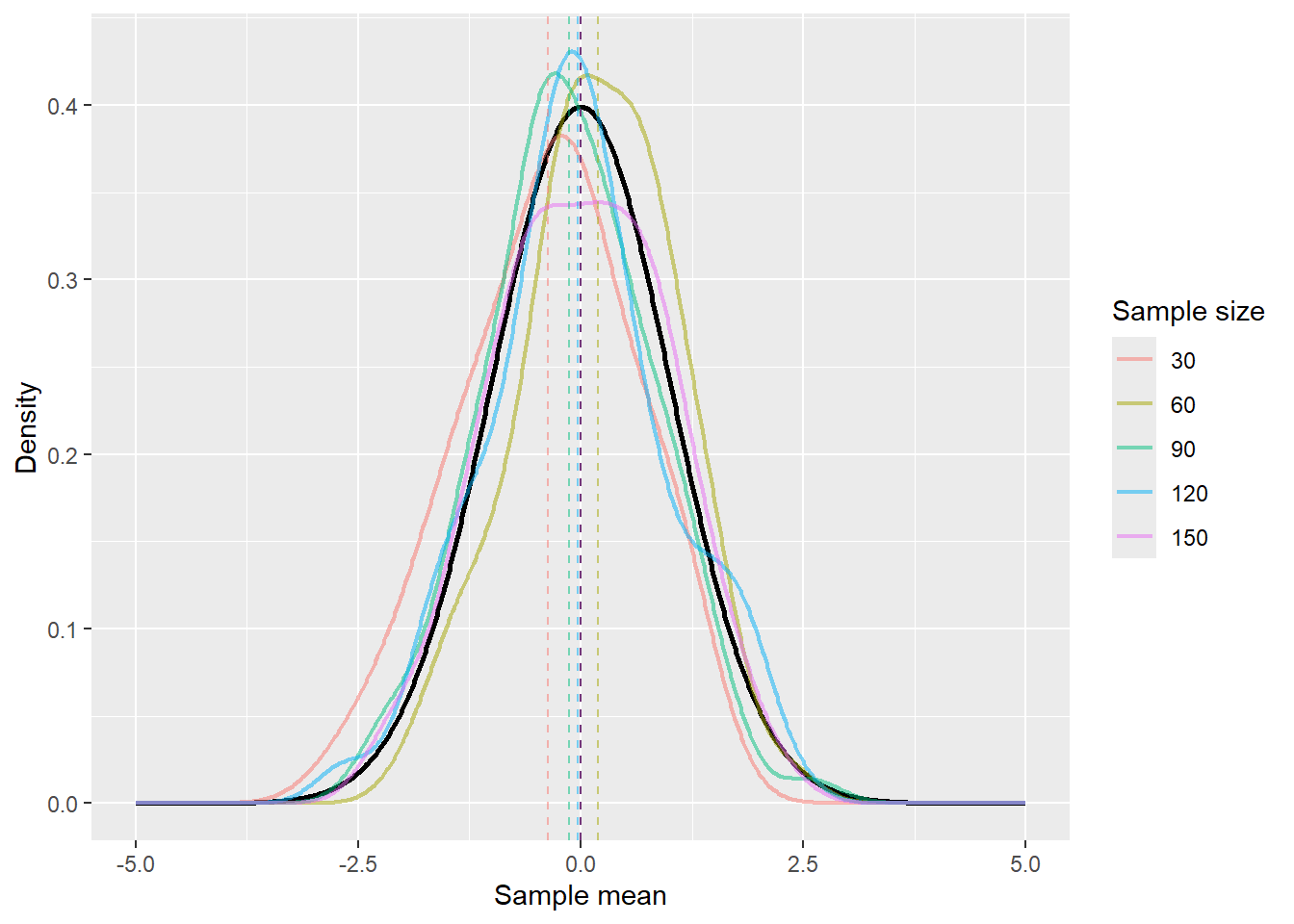
You can find excellent, vectorized code for this exact task in the QuantEcon resource.

LLN and CLT

The QuantEcon chapter on LLN and CLT provides another fantastic walkthrough with clean, professional Python code. We'll use it to guide our CLT implementation.

Focus on the section 'Simulation 1'. This provides a complete, well-commented script for demonstrating the CLT with an exponential distribution. You can adapt this code for your own implementation. Notice how it uses vectorized operations (data.mean(axis=1)) for efficiency instead of an explicit Python loop.

Density Plot of Sample Means for Various Sample Sizes — This plot demonstrates the effect of sample size `n` on the sampling distribution of the mean. As `n` increases (from 30 to 150), the distribution becomes tighter and more concentrated around the true mean, visually confirming that the variance of the sampling distribution decreases as `n` increases.

Challenge: Pushing the Boundaries

The classic LLN and CLT rely on the assumption that the samples $X_{1}, \dots, X_{n}$ are independent and identically distributed (i.i.d.). What happens if we relax the independence assumption?

Optional Challenge Task:

Consider a simple time-series model, the autoregressive process of order 1 (AR(1)):
$X_{t + 1} = α + β X_{t} + σ ϵ_{t}$
where $ϵ_{t} \sim N (0, 1)$ are i.i.d. noise terms, and $∣ β ∣ < 1$ . In this model, $X_{t + 1}$ clearly depends on $X_{t}$ , so the sequence is not independent.

The QuantEcon resource you reviewed contains an exercise about this exact case. Try to implement the simulation described in Exercise 20.3 (solution provided in section [4] of resource LINK). Does the Law of Large Numbers still appear to hold? This explores a more advanced concept known as Ergodicity, which is central to time-series analysis and connects to your engineering background in dynamical systems.

Conclusion

In this project-based lesson, you have brought the two fundamental pillars of statistical theory to life through computation.

Key Takeaways:

Law of Large Numbers: You visualized how the sample mean $X ˉ_{n}$ is a random variable that converges to a single point (the population mean $μ$ ) as the sample size n increases.
Central Limit Theorem: You demonstrated that the distribution of sample means itself converges to a specific shape—the normal distribution—centered at the population mean $μ$ with a variance of $σ^{2} / n$ . Crucially, this holds even for highly non-normal populations.
Practical Implications: These simulations show why we can trust a sample mean from a large enough sample. The LLN guarantees it's likely close to the true mean, and the CLT tells us the distribution of the error around that mean, allowing us to perform statistical inference.

Preview of the Next Module:

This lesson serves as a perfect bridge to our next topic. We have spent this module understanding the behavior of samples drawn from a population with known parameters. But in the real world, we rarely know $μ$ or $σ$ . The entire purpose of data collection is to estimate them.

In our next module, "Foundations of Statistical Inference," we will begin this quest. Our first lesson will formally introduce the concepts of estimators and explore the properties that make an estimator "good"—namely, its bias, variance, and consistency.

Recommended resources