Linear Combinations of Independent Gaussian Random Variables

1. The Power of Transforms: A Quick Review

In our study of the Central Limit Theorem, we introduced the characteristic function (CF), ${\varphi }_X(t)=\mathbb{E}[e^{itX}]$, as a powerful analytical tool. Its most crucial property for our purposes is how it behaves with sums of independent random variables.

Let's watch a brief video to refresh our memory on this key property.

This multiplicative property is the engine of our first proof. A close relative of the characteristic function is the moment-generating function (MGF), defined as $M_X(t)=\mathbb{E}[e^{tX}]$. It shares the same multiplicative property for independent variables, $M_{X+Y}(t)=M_X(t)M_Y(t)$, and is often simpler to work with as it avoids complex numbers.

For a Gaussian random variable $X\sim \mathcal{N}(\mu ,{\sigma }^2)$, the MGF is:
$M_X(t)=\exp \left(\mu t+\frac{1}{2}{\sigma }^2{t}^2\right)$
The corresponding characteristic function is ${\varphi }_X(t)=\exp \left(i\mu t-\frac{1}{2}{\sigma }^2{t}^2\right)$. Notice the similar structure.

The final piece we need is the uniqueness property: If two random variables have the same MGF (or CF) in a region around $t=0$, they must have the same probability distribution. Our strategy is simple: find the MGF of a linear combination of Gaussians and see if it matches the MGF of another Gaussian.

2. The Proof via Moment-Generating Functions

Let's prove the main result. Suppose we have $n$ independent random variables, $X_i\sim \mathcal{N}({\mu }_i,{\sigma }_i^2)$ for $i=1,\dots ,n$. We want to find the distribution of their linear combination:
$Y={\sum }_{i=1}^n{a}_i{X}_i$
where $a_i$ are constants.

We will find the MGF of $Y$, $M_Y(t)$.

1. Definition of MGF:
   $M_Y(t)=\mathbb{E}[e^{tY}]=\mathbb{E}\left[e^{t{\sum }_{i=1}^n{a}_i{X}_i}\right]$

2. Properties of Exponentials:
   $M_Y(t)=\mathbb{E}\left[{\prod }_{i=1}^n{e}^{t{a}_i{X}_i}\right]$

3. Independence: Because the $X_i$ are independent, the random variables $e^{t{a}_i{X}_i}$ are also independent. The expectation of a product of independent variables is the product of their expectations.
   $M_Y(t)={\prod }_{i=1}^n\mathbb{E}\left[e^{(a_{i}t)X_i}\right]$

4. Relating to the MGF of $X_i$: The term inside the product is the MGF of $X_i$ evaluated at the point $(a_{i}t)$.
   $\mathbb{E}\left[e^{(a_{i}t)X_i}\right]=M_{X_i}(a_{i}t)$

5. Substituting the Gaussian MGF: We know $M_{X_i}(s)=\exp ({\mu }_{i}s+\frac{1}{2}{\sigma }_i^2{s}^2)$. Substituting $s=a_{i}t$:
   $M_{X_i}(a_{i}t)=\exp \left({\mu }_i(a_{i}t)+\frac{1}{2}{\sigma }_i^2(a_{i}t{)}^2\right)$

6. Putting It All Together:
   $M_Y(t)={\prod }_{i=1}^n\exp \left(a_i{\mu }_{i}t+\frac{1}{2}{a}_i^2{\sigma }_i^2{t}^2\right)$
   When we multiply exponentials, we add their arguments:
   $M_Y(t)=\exp \left({\sum }_{i=1}^n(a_i{\mu }_{i}t)+{\sum }_{i=1}^n\left(\frac{1}{2}{a}_i^2{\sigma }_i^2{t}^2\right)\right)$
   $M_Y(t)=\exp \left(\left({\sum }_{i=1}^n{a}_i{\mu }_i\right)t+\frac{1}{2}\left({\sum }_{i=1}^n{a}_i^2{\sigma }_i^2\right)t^2\right)$

7. Conclusion: Look closely at this final form. It is the MGF of a Gaussian random variable with:

   • Mean: ${\mu }_Y={\sum }_{i=1}^n{a}_i{\mu }_i$
   • Variance: ${\sigma }_Y^2={\sum }_{i=1}^n{a}_i^2{\sigma }_i^2$

By the uniqueness property of MGFs, we have proven that $Y$ must be a Gaussian random variable with this mean and variance.

The following resource provides an excellent and concise summary of this proof strategy.

3. Alternative Perspectives and Intuition

While the MGF proof is clean and powerful, it can feel abstract. Let's explore other ways to understand this fundamental property.

The Geometric Argument

This approach provides a beautiful intuition, especially for the sum of two independent standard normal variables, $X,Y\sim \mathcal{N}(0,1)$.

The joint PDF of $X$ and $Y$ is:
$f_{X,Y}(x,y)=f_X(x)f_Y(y)=\frac{1}{\sqrt{2\pi }}{e}^{-x^2/2}\cdot \frac{1}{\sqrt{2\pi }}{e}^{-y^2/2}=\frac{1}{2\pi }{e}^{-(x^2+y^2)/2}$
The key insight is that the term $x^2+y^2$ represents the squared distance from the origin in the $xy$-plane. This means the joint PDF is radially symmetric; its value only depends on the distance from the origin, not the angle. The contours of this 3D bell-shaped surface are circles.

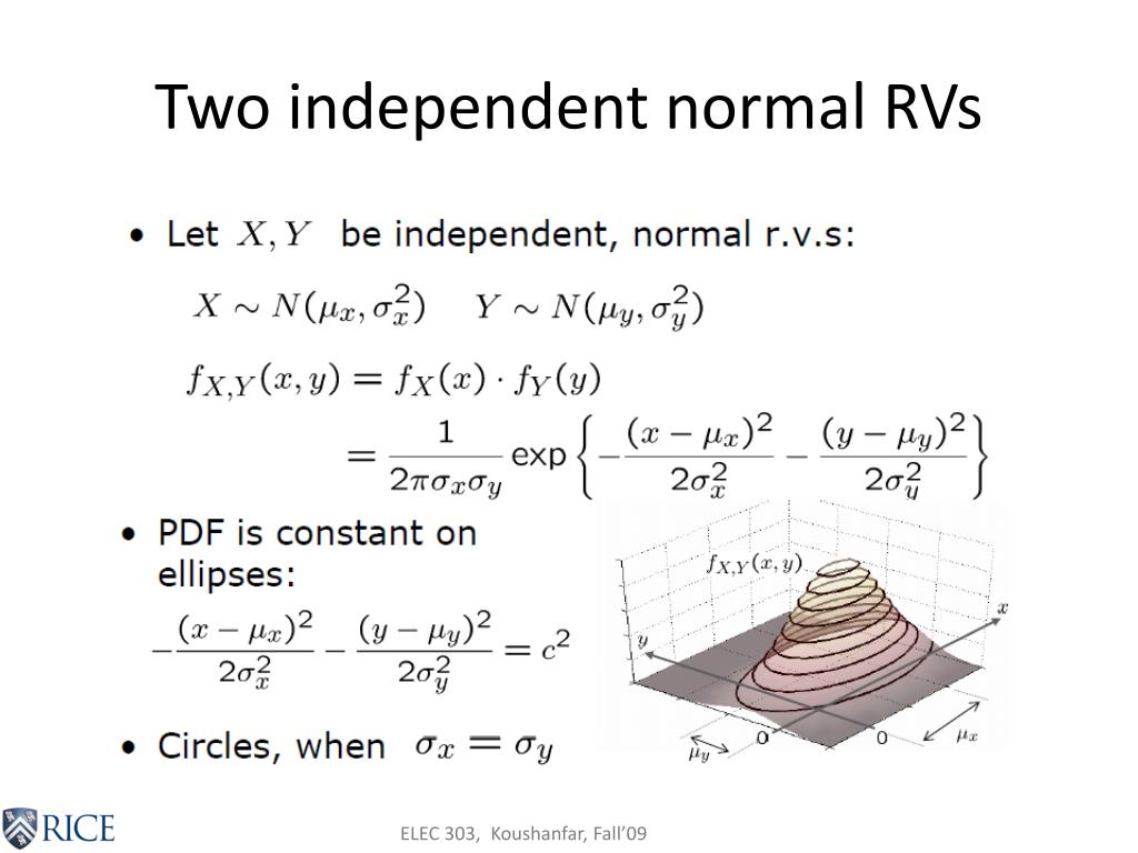
To find the distribution of $Z=X+Y$, we would normally integrate the joint PDF over the region where $x+y\le z$. However, because of the radial symmetry, we can rotate the coordinate system without changing the PDF's value at any point. Let's rotate the axes so the line $x+y=z$ becomes a simple vertical line in the new coordinate system, $x^{\prime }=c$.

The distance $c$ of this line from the origin can be found using simple geometry. The closest point on the line $x+y=z$ to the origin is $(z/2,z/2)$, so the distance is $c=\sqrt{(z/2{)}^2+(z/2{)}^2}=z/\sqrt{2}$.

After rotation, the integral for the CDF of $Z$ becomes trivial, as we are integrating a standard 2D Gaussian over the half-plane $x^{\prime }\le z/\sqrt{2}$. This simplifies to a 1D integral of a standard Gaussian, whose result is $\Phi (z/\sqrt{2})$, where $\Phi$ is the CDF of a $\mathcal{N}(0,1)$ variable. This is exactly the CDF of a $\mathcal{N}(0,2)$ variable. Thus, $X+Y\sim \mathcal{N}(0,2)$. This argument can be extended to general linear combinations.

The Convolution Proof

Another direct method is to use the formula for the distribution of a sum of independent random variables: the convolution of their PDFs.
$f_{X+Y}(z)={\int }_{-\infty }^{\infty }{f}_X(x)f_Y(z-x)dx$
Plugging in the Gaussian PDFs for $f_X$ and $f_Y$ leads to a large integral. The trick to solving it is to combine the exponents and "complete the square" for the variable of integration, $x$. This is algebraically intensive but demonstrates the result from first principles in the probability space, rather than the transform space.

The Wikipedia article on this topic provides detailed proofs for all three methods we've discussed.

4. A Quick Simulation

Let's verify this property computationally. We can simulate it in Python using NumPy. Let's take two independent Gaussians, $X_1\sim \mathcal{N}(10,2^2)$ and $X_2\sim \mathcal{N}(5,3^2)$, and form the linear combination $Y=0.5X_1+2X_2$.

According to our theorem:

• ${\mu }_Y=0.5{\mu }_1+2{\mu }_2=0.5(10)+2(5)=5+10=15$
• ${\sigma }_Y^2=(0.5{)}^2{\sigma }_1^2+(2{)}^2{\sigma }_2^2=0.25(4)+4(9)=1+36=37$

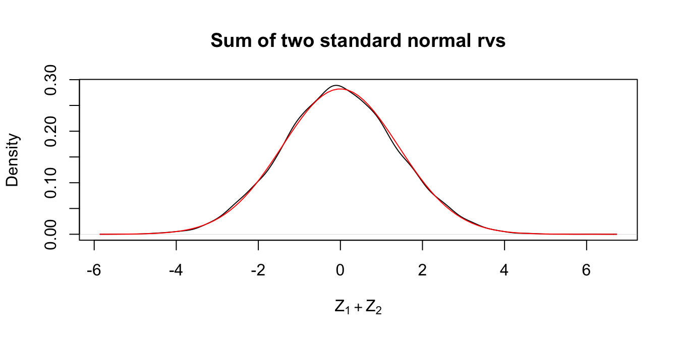
So we expect $Y\sim \mathcal{N}(15,37)$.

Here is the code to test this:

import numpy as np
import matplotlib.pyplot as plt
from scipy.stats import norm




# Parameters
mu1, sigma1 = 10, 2
mu2, sigma2 = 5, 3
a1, a2 = 0.5, 2
n_samples = 100000




# Generate samples
X1 = np.random.normal(mu1, sigma1, n_samples)
X2 = np.random.normal(mu2, sigma2, n_samples)




# Create the linear combination
Y = a1 * X1 + a2 * X2




# Theoretical parameters for Y
mu_Y = a1 * mu1 + a2 * mu2
sigma_Y_sq = a1**2 * sigma1**2 + a2**2 * sigma2**2
sigma_Y = np.sqrt(sigma_Y_sq)




# Plotting
plt.figure(figsize=(10, 6))
plt.hist(Y, bins=100, density=True, label='Simulated Data (Y)')




# Overlay the theoretical PDF
x_range = np.linspace(mu_Y - 4*sigma_Y, mu_Y + 4*sigma_Y, 200)
plt.plot(x_range, norm.pdf(x_range, mu_Y, sigma_Y), 'r-', linewidth=2, label='Theoretical PDF')
plt.title('Distribution of a Linear Combination of Gaussians')
plt.xlabel('Value')
plt.ylabel('Density')
plt.legend()
plt.grid(True)
plt.show()

print(f"Theoretical Mean: {mu_Y:.2f}, Sample Mean: {np.mean(Y):.2f}")
print(f"Theoretical Variance: {sigma_Y_sq:.2f}, Sample Variance: {np.var(Y):.2f}")

When you run this code, you'll see that the histogram of the simulated data aligns perfectly with the red line representing the theoretical Gaussian PDF, and the sample statistics will be very close to their theoretical values.

Conclusion

In this lesson, we established a critical property of the Gaussian distribution. This wasn't just an exercise in proof techniques; it was about understanding why the Gaussian distribution is so ubiquitous and analytically convenient.

Key Takeaways:

• A linear combination of independent Gaussian random variables is itself a Gaussian.
• The mean of the resulting Gaussian is the linear combination of the individual means: ${\mu }_Y=\sum a_i{\mu }_i$.
• The variance of the resulting Gaussian is a weighted sum of the individual variances, where the weights are the squares of the coefficients: ${\sigma }_Y^2=\sum a_i^2{\sigma }_i^2$.
• This property can be proven elegantly using transform methods (MGFs or CFs), which turn convolutions into simpler multiplications. Intuitive geometric arguments also exist.

Preview of the Next Lesson:

So far in this course, we have operated under the assumption that we know the parameters of our probability distributions (like $\mu$ and ${\sigma }^2$). But in the real world, these are almost never known. We only have data, and we must use that data to make educated guesses about the underlying process that generated it.

This brings us to the next major pillar of our course: Statistical Inference. In the next module, we will begin our journey into the science of estimating unknown parameters from data. Our first lesson will lay the groundwork by clearly distinguishing between the true, unknown population parameters and the sample statistics we compute to estimate them. We will then define what makes an estimator "good."