Euler's Method in Python for Equations of Motion

The Core Idea: Approximating a Curve with Straight Lines

At its heart, simulating motion is about predicting an object's path. This path is a continuous curve, but computers work in discrete steps. Euler's method provides a way to approximate this curve by taking a series of small, straight-line steps.

Imagine you know your position and velocity at a specific moment. You can make a reasonable guess about your position a fraction of a second later by assuming your velocity is constant during that tiny interval. You then repeat this process from your new position, with your new velocity, and so on.

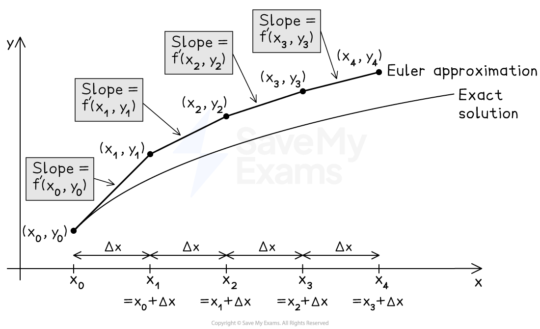
Euler's method approximates an exact solution (a smooth curve) by taking discrete steps. At each point, the slope (derivative) is used to project to the next point, creating a series of connected line segments.

This is exactly what our update equations from the last lesson do. The term $v\cdot \Delta t$ represents the small change in position over the time step $\Delta t$, which we add to the old position to get the new one.

Applying Euler's Method to Physics

For our purposes, we're solving equations based on Newton's second law, $F=ma$, which can be written as an ordinary differential equation (ODE):
$\frac{d^{2}s}{d{t}^2}=a=\frac{F}{m}$
This is a second-order ODE because it involves the second derivative of position, $s$. As a programmer, you can think of this as needing to "integrate twice" to get from acceleration back to position. We'll apply Euler's method in two steps within a loop:

1. Update Velocity: First, we use the acceleration to find the velocity at the end of the time step.
2. Update Position: Then, we use that newly calculated velocity to find the final position.

The video below gives an excellent conceptual overview of this process, showing how a second-order ODE (for a spring-mass system) is broken down into these two steps.

The update procedure described in the video is often called the Semi-Implicit Euler (or Euler-Cromer) method. Its key feature is using the velocity from the end of the timestep ($v_{n+1}$) to calculate the new position. This simple choice makes the simulation significantly more stable than using the velocity from the beginning of the timestep, a topic we'll explore in detail in the next lesson.

For now, these are the only equations you need:

1. Calculate current acceleration: $a_n=F_n/m$
2. Update velocity: $v_{n+1}=v_n+a_n\cdot dt$
3. Update position: $s_{n+1}=s_n+v_{n+1}\cdot dt$

A Simple Implementation in Python

Let's translate this directly into Python. We can simulate the 1D motion of an object in freefall. We'll set an initial position and velocity, then loop forward in time, applying our update rules until the object hits the ground. Since you're proficient with Python, the structure should feel very familiar.

# --- 1. Initialization ---
# Physical constants and initial conditions
g = 9.81        # Acceleration due to gravity (m/s^2)
pos = 100.0     # Initial position (height in meters)
vel = 0.0       # Initial velocity (m/s)

# Simulation parameters
dt = 0.1        # Time step (seconds)
t = 0.0         # Start time

# Data logging
positions = [pos]
times = [t]

# --- 2. Simulation Loop ---
while pos > 0:
    # Calculate acceleration (constant in this simple case)
    accel = -g

    # Update velocity (Euler step 1)
    vel = vel + accel * dt

    # Update position using the new velocity (Euler step 2)
    pos = pos + vel * dt

    # Update time
    t = t + dt

    # Log the data
    positions.append(pos)
    times.append(t)
    
# --- 3. Output ---
print("Simulation finished.")
print(f"Time of flight: {t:.2f} s")
print(f"Final velocity: {vel:.2f} m/s")

This short script is a complete physics simulation. At each step, it calculates the new velocity and position and adds them to a list. This iterative process, running inside a while loop, is the heart of numerical simulation. The image below shows a more advanced version that simulates projectile motion in 2D and visualizes the result, but the core logic in the while loop is exactly the same.

A Python program using Euler's method to calculate the trajectory of a projectile. The code on the left performs the iterative updates, and the graph on the right visualizes the resulting path.

From a Simple Script to a Rocket Simulation

This simple method is powerful enough to form the basis of complex simulations. To show you how this scales up to your goal of simulating rockets, let's look at a practical example. The following article details the creation of a 2D rocket simulation in Python.

The code is more complex—it uses NumPy for vector math and handles forces from thrust and gravity—but the core integration loop uses the exact same Euler method.

Notice the direct parallel between the rocket code and our simple freefall script. Both initialize variables, loop through time, calculate acceleration, and use it to update velocity and then position. This fundamental pattern is the engine that will drive all the simulations we build in this course.

You may have noticed the author of that article uses a slightly different update order: they update position using the velocity from the start of the time step. This is known as the Explicit Euler method. While it works, it is less stable than the Semi-Implicit version we are using. We will investigate the crucial difference this makes in our next lesson.

Conclusion

In this lesson, you've taken the final step from theory to practice, implementing Euler's method to solve equations of motion in Python. This is a significant milestone, as you now have the primary tool for building physics simulations.

Here are the key takeaways:

• Euler's method approximates motion by taking small, discrete time steps ($dt$).
• For physics simulations based on $F=ma$, we apply the method twice in a loop: first to update velocity from acceleration, and then to update position from velocity.
• The Semi-Implicit Euler method, which uses the newly updated velocity to calculate the new position, is generally more stable and preferred.
• The core of a simulation is a loop that repeatedly applies these update rules: $v_{n+1}=v_n+a_n\cdot dt$ and $s_{n+1}=s_n+v_{n+1}\cdot dt$.

You've seen how this simple process works in a basic script and how it scales up to a more complex rocket simulation. However, the accuracy and reliability of this method depend heavily on one key parameter: the time step, dt. In our next lesson, we will analyze the effect of dt on the accuracy and stability of our simulations.