One-Dimensional Free Fall: Modeling Gravitational Force

Welcome to Module 3! In the previous module, we explored the mechanics of numerical simulation, focusing on how to translate the calculus of motion into code with Euler's method and understanding the critical role of the time step dt. Now, we shift our focus from the "how" of simulation to the "what." We will begin applying these powerful techniques to model real physical systems, starting with the most fundamental force governing flight on Earth: gravity.

This lesson lays the groundwork for our first full simulation. We will model the forces acting on an object in 1D free fall. This simple scenario is the perfect entry point into computational physics and serves as an essential foundation for our ultimate goal of simulating a rocket's trajectory. After all, even as a rocket soars upward, gravity is relentlessly pulling it back down. By the end of this lesson, you will have a clear physical and mathematical model for gravity's effect, ready to be translated into Python code.

The Physics of Free Fall

Let's begin with a clear definition. An object is in free fall when the only force acting on it is gravity. For now, we will make a simplifying assumption that is common in introductory physics: we will ignore the effects of air resistance.

In this scenario, the force of gravity is simply the object's weight. Your high school physics background will likely remind you that weight ( $W$ ) is the product of an object's mass ( $m$ ) and the gravitational field strength, which we denote as $g$ .

W = m g

Now, let's bring in Newton's Second Law of Motion, the master equation that connects forces to motion:

F_{n e t} = ma

Where $F_{n e t}$ is the net force on the object, $m$ is its mass, and $a$ is its resulting acceleration. In free fall, the net force is the weight of the object. By substituting $W$ for $F_{n e t}$ , we arrive at a remarkably elegant conclusion.

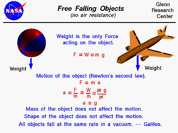
As this diagram from NASA's Glenn Research Center illustrates, when weight is the only force acting on an object, Newton's Second Law (F=ma) simplifies the motion. The force (F) is the weight (W=mg), leading to the equation ma = mg.

If we set the force equal to the weight:

ma = m g

We can divide both sides by the mass, $m$ :

a = g

This is a profound result. It shows that in a vacuum, the acceleration of a falling object is constant and, critically, independent of its mass. A feather and a bowling ball will indeed fall at the same rate, not because the force on them is the same (the bowling ball is much heavier), but because their acceleration is the same.

Understanding `g`: Acceleration and Sign Conventions

The constant acceleration $g$ is known as the acceleration due to gravity. Near the Earth's surface, its value is approximately 9.8 m/s². This means that for every second an object is in free fall, its downward velocity increases by 9.8 meters per second.

To correctly model this in a simulation, we need to define a coordinate system. In physics and engineering, it's standard to define the "up" direction as positive and the "down" direction as negative. Since gravity always pulls objects downward, its acceleration is represented with a negative sign.

a = - g = - 9.8 m/s^{2}

The following video explains this concept clearly and also provides a deeper look into the physics behind why mass cancels out.

The Acceleration of Gravity and Free-Fall Equations

This video from the "Math and Science" channel provides an excellent introduction to gravitational acceleration.

First, watch the segment that defines g and explains the sign convention for vertical motion problems: gravitational acceleration. Next, watch the fascinating explanation of why all objects fall at the same rate. The presenter uses Newton's Law of Universal Gravitation and F=ma to show mathematically why the mass of the falling object cancels out: Why objects fall together. This connects the concept of "gravitational mass" (which determines weight) and "inertial mass" (which resists acceleration).

The "Constant `g`" Assumption

For our simulations of bottle rockets and model rockets, we will assume that $g$ is a constant value of 9.8 m/s². This is a very safe and standard approximation for objects moving near the Earth's surface.

However, as you pursue your interest in aerospace, it's important to know that $g$ is technically not constant. The force of gravity weakens with distance. For simulations involving orbits or interplanetary travel, this variation is crucial and must be accounted for. The video you just watched briefly touches on this point, which is an excellent preview of the complexities involved in more advanced rocketry simulations. For our purposes, constant $g$ is the correct and appropriate model.

From a Physical Law to a Simulation Rule

We have now established our physical model: an object in 1D free fall experiences a constant downward acceleration of $a = - 9.8 m/s^{2}$ .

How do we use this in our simulation? We simply plug this constant acceleration into the Euler method equations we developed in the previous module. Recall the update rules for our semi-implicit Euler method:

Update Velocity: $v_{n e w} = v_{o l d} + a \cdot Δ t$
Update Position: $y_{n e w} = y_{o l d} + v_{n e w} \cdot Δ t$

In each step of our simulation loop, the acceleration $a$ will simply be our constant, -9.8. This is the core of modeling gravity for vertical motion. The following resource provides a concise walkthrough of this exact logic.

Physics Undergraduate Practicals

This guide from the University of Toronto practicals walks through the process of setting up a numerical integration for free fall. It directly connects the physics to the step-by-step update equations.

Please read the section titled "Numerical Integration". Start from the text that introduces the update equations. Notice how it explicitly derives v(t + dt) and x(t + dt), which are the exact rules we will implement in our simulation loop.

A Note on Analytical vs. Numerical Solutions

For the special case of constant acceleration, it's possible to find the exact position and velocity of an object at any time using a set of formulas called the kinematic equations. This is known as an analytical solution.

Our simulation, which calculates the motion step-by-step, is a numerical solution.

In a future lesson, we will compare our numerical simulation results against the analytical solution given by these equations to verify the accuracy of our code. For now, it's useful to be aware that these equations exist.

Free Fall Physics Problems - Acceleration Due To Gravity

This video by "The Organic Chemistry Tutor" introduces the standard kinematic equations used for constant acceleration problems.

Watch the short segment from this point to familiarize yourself with the four main kinematic equations. You don't need to memorize them, but recognize that they provide a direct, non-iterative way to solve free-fall problems.

Understanding the difference between these two approaches is key. While analytical solutions are exact, they only exist for relatively simple systems. The power of numerical simulation, which you are learning, is that it can be applied to far more complex problems where no exact formula exists—like a rocket flight with changing mass and variable air resistance.

Conclusion

In this lesson, we established the fundamental model for 1D motion under gravity. We've taken a physical principle and translated it into a clear set of rules ready for computation.

Here are the key takeaways:

In free fall (neglecting air resistance), the only force on an object is its weight ( $W = m g$ ).
Applying Newton's Second Law ( $F = ma$ ), we find that all objects in free fall have the same constant downward acceleration, $a = g$ , which is approximately 9.8 m/s².
For our simulation's coordinate system, we model this as $a = - 9.8 m/s^{2}$ .
This constant acceleration is the key input for the Euler method update rules that will drive our simulation.

You have now defined the physics. In our next lesson, we will take this model and bring it to life, writing a complete Python simulation of an object in 1D free fall.

Recommended resources