Welcome back! In our last lesson, we established that the integral represents an accumulated sum, which can be visualized as the area under a curve. We also touched on the crucial idea that the update rules in a simulation are a practical application of this concept, a method called a Riemann Sum.
Today, we will solidify that connection by exploring the precise physical relationships that integration governs. Your goal is to learn how to relate integration to finding displacement from velocity, and in turn, velocity from acceleration. This is the inverse of the differentiation we studied earlier and forms the theoretical backbone of how we'll build our motion simulation. By the end of this lesson, you'll understand not just the "what" of integration, but the "why" for simulating physics.
The Inverse Relationship: From Acceleration to Position
In a previous lesson, we saw that if you have a position-time graph, taking the derivative (finding the slope) gives you the velocity. Taking the derivative of the velocity graph gives you the acceleration. So, how do we go the other way? If we know an object's acceleration—perhaps from the force of a rocket motor—how can we determine its velocity and final position?
The answer is integration. Integration and differentiation are inverse operations; one undoes the other.

This means:
- Velocity is the integral of acceleration with respect to time.
- Displacement is the integral of velocity with respect to time.
Let's see how this works in practice with a formal calculus example. The following video walks through a problem where, given an acceleration function, the host uses integration twice to find the velocity and position functions.
Velocity and Position From Acceleration By Integration - Physics and Calculus
This video from The Organic Chemistry Tutor provides a clear, step-by-step demonstration of analytical integration to solve a kinematics problem.
Watch the entire video. Pay attention to how: The acceleration function is integrated to get a velocity function (integrating acceleration). An initial condition (V(1) = 10) is used to solve for the constant of integration, C (finding C for velocity). The resulting velocity function is integrated to find the position function (integrating velocity). Another initial condition (X(2) = 17) is used to find the new constant of integration (finding C for position).
This process of finding the "antiderivative" is the formal, analytical way to perform integration. However, for our simulations, especially when forces (and thus accelerations) are complex and changing, we will rely on the numerical approach we discussed last time: summing up small changes over time.
Physical Interpretation: The Area Under the Velocity-Time Graph
Let's connect this back to the idea of the integral as the "area under a curve." Look at the velocity-time graph below.
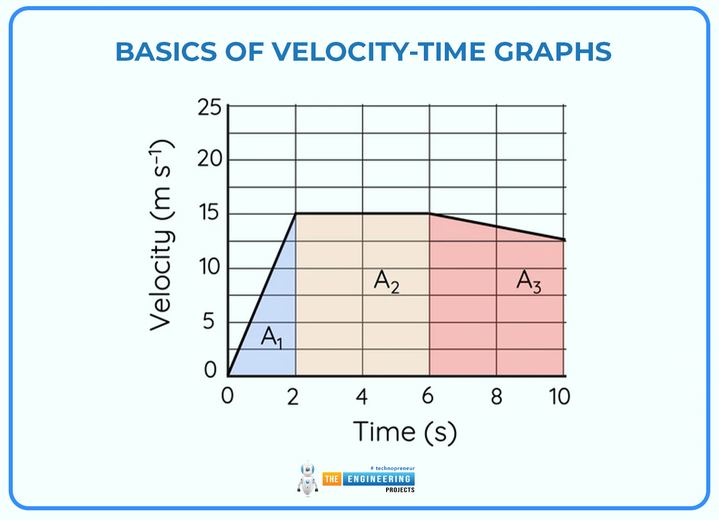
In the previous lesson, we established that the area under this curve represents the total distance traveled. This is the physical meaning of integrating velocity.
- The area is calculated as "height" × "width," which corresponds to "velocity" × "time." The units confirm this: , the unit of displacement.
- The total displacement over the 10 seconds shown is the sum of the areas of the three shaded regions: (a triangle), (a rectangle), and (a trapezoid).
Similarly, if this were an acceleration-time graph, the area under the curve would represent the change in velocity. This is the core principle we'll use. We'll calculate the tiny change in velocity over a small time step and add it to the current velocity. Then, we'll use that new velocity to calculate the tiny change in position and add it to the current position, repeating this process over and over.
The following resource from UNSW Physics formalizes this relationship using the language of definite integrals.
Integration of displacement, velocity and acceleration
This video explains how the integral equations for velocity and displacement are set up from their derivative definitions.
Please watch the first two conceptual segments: The derivation for velocity from acceleration: Velocity from acceleration The derivation for displacement from velocity: Displacement from velocity Notice how the limits of integration correspond to the initial and final states (e.g., from an initial time t_i to a final time t_f).
From Continuous Integration to Discrete Simulation
So, how do we apply this in a computer program? A computer can't work with the smooth, continuous functions of pure calculus. It works in discrete steps. This is where numerical integration comes in.
The following document was created for a course on game physics, but the principles are identical for our rocket simulation. It explicitly lays out the practical steps of building a physics engine based on integration.
Physics Tutorial 2: Numerical Integration Methods
This document bridges the gap between the calculus theory and the implementation in a simulation. It shows how the continuous idea of an integral is turned into discrete update equations.
Please read the following sections: Start with the section on "Linear Motion" (p. 1). This reinforces the core relationships: v = ∫ a dt and s = ∫ v dt. Next, read the brief paragraph on the informal definition of integration as the "area under the trace" (p. 2). Now, look at the steps for a "Force-Based Physics Engine" (p. 3). Notice how "Integrate the acceleration" and "Integrate the velocity" are key steps. Finally, read the section on "Explicit Euler Integration" (p. 4). This is the crucial part. Look at the two equations presented: v_{n+1} = v_n + a_n \Delta t s_{n+1} = s_n + v_n \Delta t
These two equations are the heart of our next lesson and our future simulations. They are the direct, practical implementation of the integration concepts we've discussed:
- The term represents the area of a small rectangle under the acceleration-time graph over a small time interval . It's the small change in velocity during that step. By adding it to the old velocity , we get the new velocity . We have just integrated acceleration to find velocity.
- Similarly, is the area of a small rectangle under the velocity-time graph. It's the small change in position. By adding it to the old position , we get the new position . We have just integrated velocity to find displacement.
Repeating these two steps in a loop is how we simulate motion through time.
Conclusion
In this lesson, we've connected the abstract concept of integration to the concrete physics of motion. We've seen how this one mathematical tool is the key to working backward from forces and acceleration to determine an object's trajectory.
Here are the main takeaways:
- Integration is the inverse of differentiation. Just as we can find velocity by differentiating position, we can find displacement by integrating velocity.
- The fundamental relationships for our simulation are: velocity is the integral of acceleration, and displacement is the integral of velocity.
- In a numerical simulation, we perform integration step-by-step. The update rules and are the direct computational forms of these integral relationships.
You now have all the conceptual tools needed to build a simulation. You understand how to find rates of change (derivatives) and how to accumulate those changes over time (integrals). In our next lesson, we will finally dive into the code and implement Euler's method, using the very update equations you saw today to build a Python program that simulates an object's motion.