Welcome to the next lesson in our journey to build a rocket simulation. Last time, we explored how the derivative gives us the instantaneous rate of change, allowing us to find velocity from position, and acceleration from velocity. We saw that this relationship is the key to creating update rules for a simulation.
Today, we'll learn about the other side of that coin: integration. If derivatives help us break down motion into instants, integrals help us build it back up by accumulating changes over time. Your goal for this lesson is to define the integral as the accumulated sum of a quantity and relate this concept to finding the area under a curve. This is the final piece of the conceptual puzzle we need before we start writing our first physics simulation.
From Velocity to Position: The Inverse Problem
In our last lesson, we looked at graphs like the one below and saw that the slope of the position curve (blue) gives the value of the velocity curve (green), and the slope of the velocity curve gives the value of the acceleration curve (red).

This is differentiation. But what if we start with a known acceleration (caused by forces like gravity or a rocket motor) and want to figure out the resulting velocity and position? We need to go in reverse. This means asking questions like: "If I know my velocity at every moment, how far have I traveled?" This reverse process is called integration.
The following video from 3Blue1Brown provides a beautiful, intuitive explanation of this exact problem, framing it as finding the distance a car has traveled by only looking at its speedometer.
Integration and the fundamental theorem of calculus | Chapter 8, Essence of calculus
This video masterfully introduces the concept of integration by connecting it to the familiar problem of determining distance from a varying velocity.
Please watch from the beginning up to the point where the connection between distance traveled and the area under a velocity-time graph is made. Pay close attention to the logic: How distance is calculated for a constant velocity (constant velocity case). How this corresponds to the area of a rectangle on the graph (visualizing distance as area). What makes the problem difficult when velocity changes continuously (the challenge).
Approximating the Area Under a Curve
As you just saw, the total distance traveled is equivalent to the area under the velocity-time graph. This is a profound insight. For a constant velocity, the area is a simple rectangle. But what about a curve?
The core idea of integration is to solve this problem through approximation. We slice the area under the curve into many thin shapes that we do know how to calculate the area of, like rectangles. We then sum up the areas of all these small shapes. The more, and thinner, the rectangles we use, the better our approximation gets.
This method of summing up the areas of rectangles is called a Riemann Sum. Let's see it in action with a concrete numerical example.
What is Integration? Finding the Area Under a Curve
In this video, Professor Dave Explains provides a clear, step-by-step example of how to approximate the area under a curve using rectangles.
Please watch the first three sections of the video, which cover: The problem of finding the area under a curve (introduction). The strategy of approximating with rectangles (the approximation). A quantitative example showing how the approximation improves as you add more rectangles (numerical example).
The Integral as an Accumulated Sum
The process you've just seen is the heart of today's learning outcome. The integral is defined as the accumulated sum of a quantity. By adding up the areas of all the small rectangles (), we are accumulating the total distance traveled over the entire interval.
As the width of these rectangles, which we can call , becomes infinitesimally small (approaching zero), our approximation becomes perfectly accurate. This limit of the Riemann sum is what we call the definite integral.
The blog post below provides an excellent summary of this idea and even shows you how it can be implemented in Python.
Integrals are Easy: Visualized Riemann Integration in Python | iSquared
This article does a great job of building the concept from intuition to a formal definition, and even provides a more accurate method using trapezoids.
Please read the first three main sections of the article: "Intuition": Start by reading the introductory section, which reinforces the idea of approximating an irregular area with simple rectangles. "Riemann Integration Definition": Continue to the next section. This part formalizes the sum of rectangles and introduces an improvement: using trapezoids instead of rectangles for a better fit.
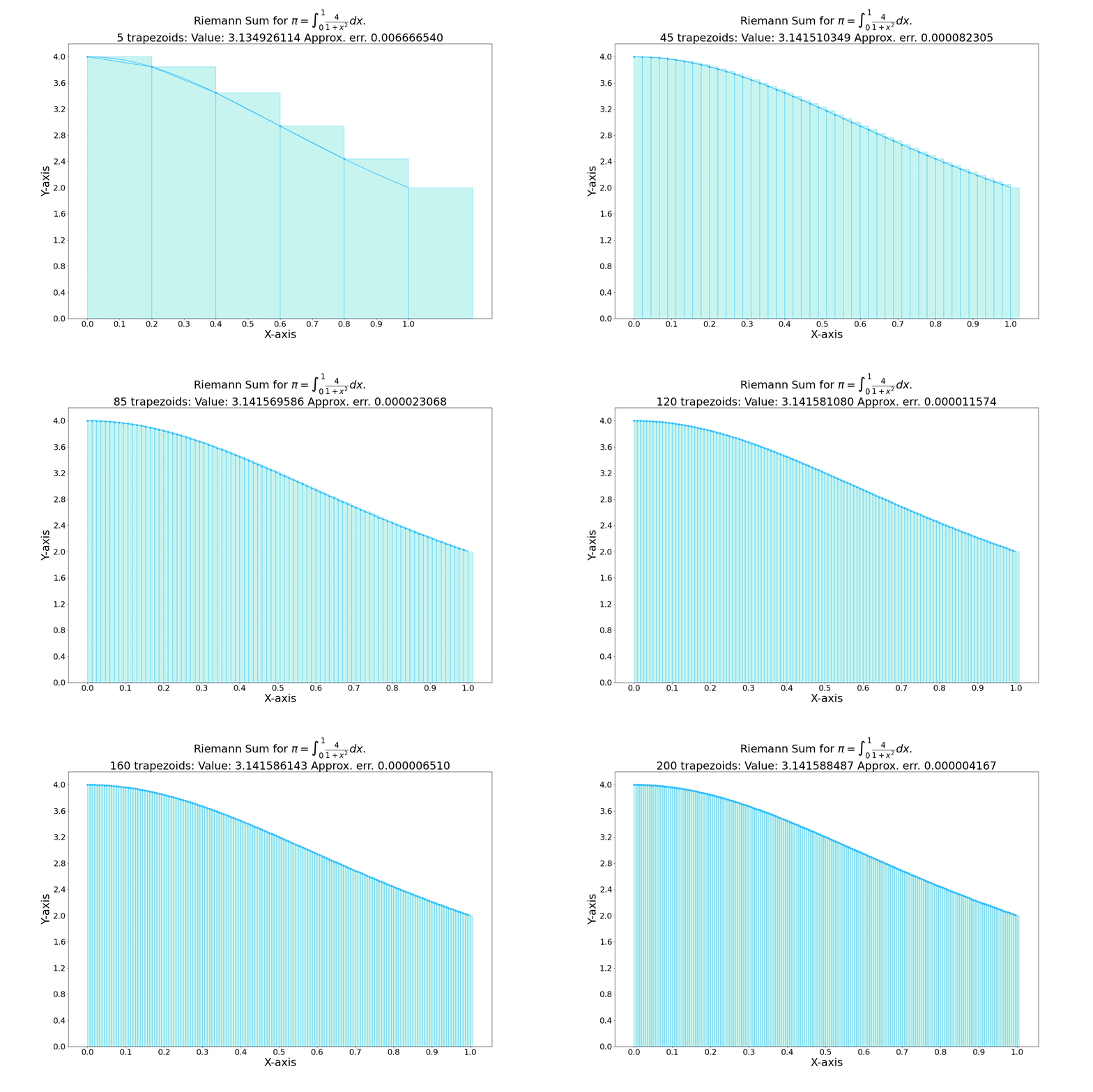
The animated image below, taken from that article, perfectly illustrates this process. As the number of shapes (trapezoids, in this case) increases, their combined area becomes a near-perfect match for the area under the curve.
Connecting Integration to Simulation
So, how does this all relate to our goal of simulating a rocket?
In a computer simulation, we can't make our time step infinitely small. Instead, we choose a very small, but finite, time step, often called dt. Our simulation loop then calculates the state of our rocket at each step.
Remember the update rules from our last lesson?
new_velocity = old_velocity + acceleration * dtnew_position = old_position + velocity * dt
Look closely at the first rule. acceleration * dt is the change in velocity over that tiny time step. It's the area of one thin rectangle on an acceleration-vs-time graph. By adding this small area to our old_velocity, we are performing one step of a Riemann sum! We are integrating acceleration to find velocity.
The same applies to the second rule. velocity * dt is the area of a thin rectangle on a velocity-vs-time graph. By adding it to old_position, we are integrating velocity to find position.
So, a numerical simulation is, in essence, a step-by-step process of performing a Riemann sum. The "accumulated sum" is not just a mathematical abstraction; it is the literal process by which our simulation will calculate the rocket's trajectory over time.
Conclusion
In this lesson, we've uncovered the second fundamental tool of calculus for our simulation toolkit. You now understand the integral in a way that is directly applicable to coding physics.
Here are the key takeaways:
- Integration is the process of accumulating a quantity over an interval.
- This can be visualized as finding the area under the curve of a graph.
- We can approximate this area by summing up many small rectangles or trapezoids, a method known as a Riemann Sum.
- The definite integral is the exact value that this sum approaches as the slices become infinitely thin.
- Crucially for us, the update rules in a time-step simulation are a practical implementation of a Riemann sum, integrating acceleration to get velocity, and velocity to get position.
We now have the two pillars of calculus needed for our simulation: differentiation to determine rates of change from forces, and integration to accumulate those changes into motion. In our next lesson, we will put this all together and implement Euler's method, a straightforward technique for numerically solving equations of motion based on the very principles we've just discussed.