The Derivative as Instantaneous Rate of Change

From Average Speed to Instantaneous Speed

You're already familiar with the idea of a rate of change from your physics background. When you calculate a car's speed by dividing the distance traveled by the time it took, you are finding its average speed.

Average Speed = (Change in Position) / (Change in Time)

This gives you a single number for the entire trip. But what if you want to know your speed at one specific moment—the speed your car's speedometer shows? That's the instantaneous speed. The derivative is the mathematical tool for finding exactly this: the rate of change at a single instant.

The following article uses this speedometer analogy to build a fantastic intuition for what a derivative represents.

This idea of shrinking the time interval is the conceptual leap from algebra to calculus. To find the rate of change at a single point, we start by calculating the average rate over a small interval around that point and then imagine making that interval infinitely small.

A Geometric View: Slope of the Tangent Line

We can visualize this concept on a graph. For a straight line, the slope is constant; the rate of change is the same everywhere. But for a curve, like the trajectory of a rocket, the steepness—and thus the rate of change—is constantly varying.

The average rate of change between two points on a curve is simply the slope of the straight line connecting them. This line is called a secant line.

To find the instantaneous rate of change at a single point, we can imagine moving the two points of the secant line closer and closer together. As the distance between the points approaches zero, the secant line pivots to become the tangent line—a line that just touches the curve at that one point. The slope of this tangent line is the derivative at that point.

The following video from Khan Academy explains this geometric interpretation very clearly.

This next short, animated video provides a dynamic visualization of a secant line transforming into a tangent line. This visual can be very helpful for cementing the concept.

The image below summarizes this entire process. On the left, we calculate an average rate of change over a noticeable interval, $\Delta x$. On the right, we see what happens as we shrink that interval towards zero: the average rate becomes the instantaneous rate at a single point.

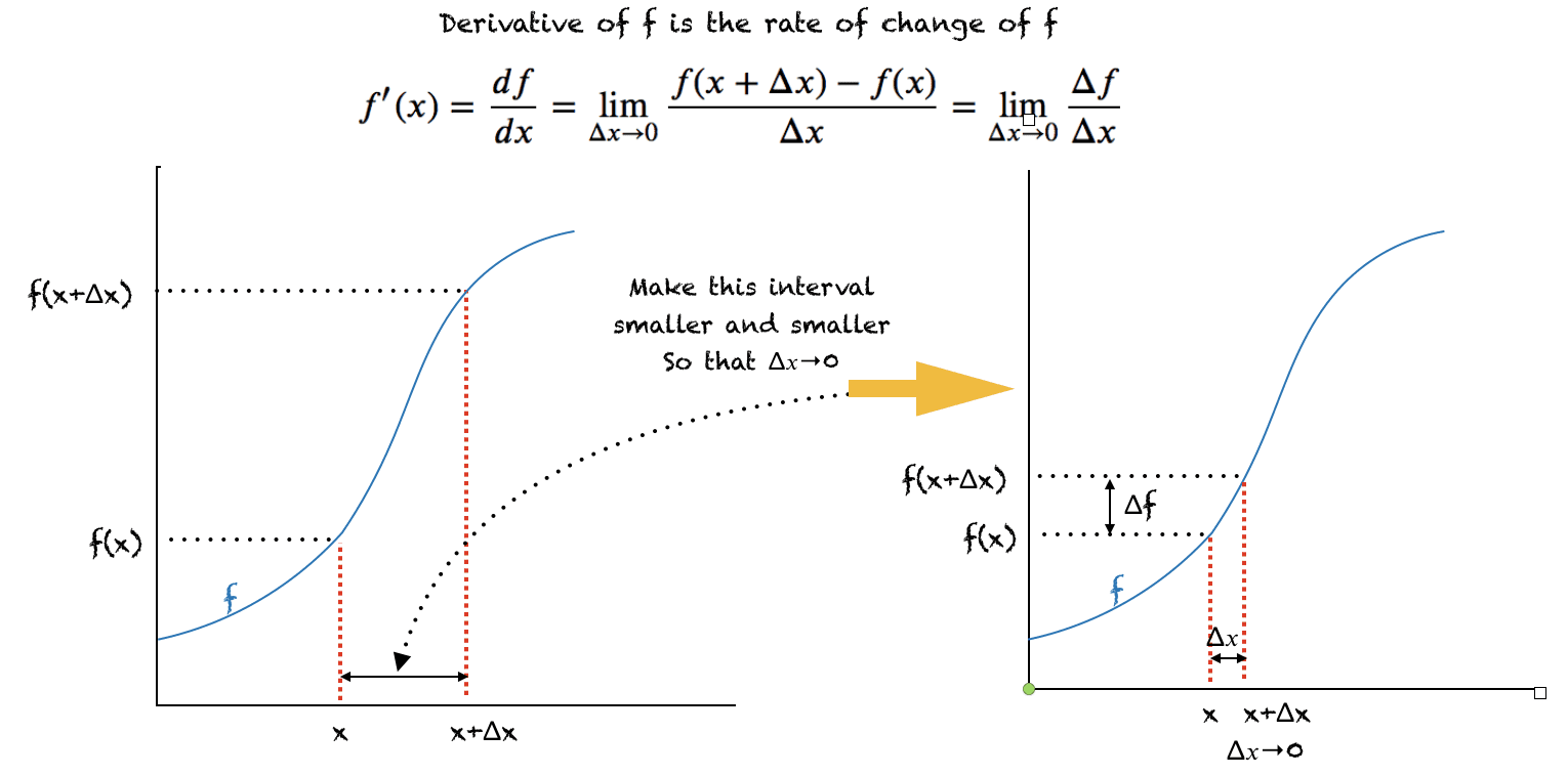
A visual representation of the derivative. The average rate of change between $x$ and $x+\Delta x$, given by the slope of the secant line, approaches the instantaneous rate of change at $x$, given by the slope of the tangent line, as the interval $\Delta x$ shrinks to zero.

The Formal Definition and Numerical Approximation

Mathematically, this process of "shrinking the interval to zero" is called taking a limit. The formal definition of the derivative of a function $f(x)$, denoted as $f^{\prime }(x)$ (read "f prime of x"), is:

Let's break this down:

• $f(x)$ is the value of your function at some point $x$.
• $\Delta x$ (delta x) is a small change in the input, our "interval".
• $f(x+\Delta x)$ is the value of the function a small step away.
• The numerator, $f(x+\Delta x)-f(x)$, is the change in the function's value, which we can call $\Delta f$.
• The fraction $\frac{\Delta f}{\Delta x}$ is the average rate of change over that small interval (rise over run).
• The ${\lim }_{\Delta x\to 0}$ part means we are finding the value that this fraction approaches as our interval $\Delta x$ gets infinitesimally small. This gives us the instantaneous rate of change.

Another common notation for the derivative, introduced by Leibniz, is $\frac{dy}{dx}$. This notation is very evocative of its origin as the limit of $\frac{\Delta y}{\Delta x}$.

For our rocket simulations, we can't make the time step $\Delta t$ infinitely small. Instead, we will do what the definition implies: we'll make it very small. This gives us a numerical approximation of the derivative, which is perfect for a step-by-step computer simulation.

This next resource provides a concise walkthrough of this idea, complete with a Python implementation.

Let's look at the Python function from that article. It's an implementation of the forward difference method, a common way to approximate a derivative.

import numpy as np

def f(x):
  """A simple quadratic function for demonstration."""
  return x**2

def approximate_derivative(func, x, h):
  """
  Calculates the approximate derivative of a function at a point x.
  
  Args:
    func: The function to differentiate (e.g., f).
    x: The point at which to find the derivative.
    h: A very small step size (our delta_x).
    
  Returns:
    The approximate derivative at x.
  """
  return (func(x + h) - func(x)) / h

# --- Calculate the derivative of f(x) = x^2 at x = 2 ---
x_point = 2
h = 1e-6 # A small step size, equivalent to 0.000001

# Calculate the approximation
deriv_at_2 = approximate_derivative(f, x_point, h)

print(f"The function is f(x) = x^2")
print(f"The approximate derivative at x = {x_point} is: {deriv_at_2}")

# The exact analytical derivative of x^2 is 2x. At x=2, the exact derivative is 4.
# Our approximation is very close!

This simple function is incredibly powerful. It can find the instantaneous rate of change for any function func you give it, at any point x. This is the core mechanism we will use to update our rocket's state in our simulations. By knowing the rocket's position at one moment, we can calculate its velocity (the derivative of position), and use that to predict its position a fraction of a second later.

Conclusion

In this lesson, you have been introduced to the fundamental concept of the derivative. We moved from an intuitive understanding to a precise mathematical definition, and finally to a practical implementation in code.

Here are the key takeaways:

• A derivative measures the instantaneous rate of change of a function at a specific point.
• Geometrically, the derivative is the slope of the tangent line to the function's graph at that point.
• The derivative is formally defined as the limit of the average rate of change ($\frac{\Delta y}{\Delta x}$) as the interval ($\Delta x$) shrinks to zero.
• In simulations, we approximate the derivative numerically by using a very small but finite step size, $h$.

You now have the primary mathematical tool needed to describe motion. In the next lesson, we will apply this concept directly to the physics of our simulation. We will formally define velocity as the derivative of position with respect to time, and acceleration as the derivative of velocity with respect to time. This connection is the heart of simulating motion and will be our next step toward building our rocket simulation.

A preview of our next topic: the relationships between position, velocity, and acceleration, which are mathematically defined by derivatives.