Comparing Flight Parameters with Multi-Dataset Plots

Method 1: Multiple Lines on the Same Axes

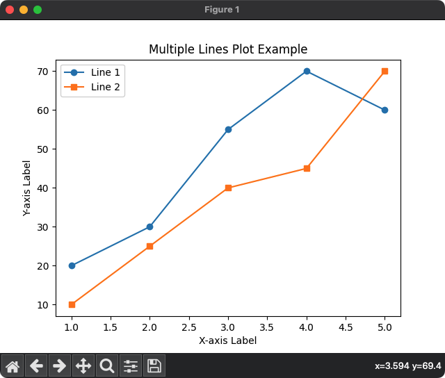
In the last lesson, you saw that you can plot multiple lines by simply calling plt.plot() several times before plt.show(). This is the most direct way to compare datasets that share the same units or have similar scales, like comparing the median salaries for different developer roles.

The following video from Corey Schafer provides an excellent, practical walkthrough of this technique. It reinforces what you've learned and adds important details about customizing lines to make your plots more readable.

Let's apply this to a simple flight scenario. Imagine we have data for a rocket's altitude and its velocity during the first few seconds of ascent. Both are measured against time.

import numpy as np
import matplotlib.pyplot as plt




# --- 1. Generate Sample Flight Data ---
time = np.linspace(0, 10, 100) # Time from 0 to 10 seconds




# Simplified kinematics (these are not from a real simulation yet)
# Altitude increases quadratically (like s = 1/2*a*t^2)
altitude = 2.5 * time**2




# Velocity increases linearly (like v = a*t)
velocity = 5 * time




# --- 2. Create the Plot ---
plt.figure(figsize=(10, 6)) # Create a figure with a nice size




# Plot altitude vs. time
plt.plot(time, altitude, label="Altitude (m)", color="blue", linestyle="-")




# Plot velocity vs. time on the same axes
plt.plot(time, velocity, label="Velocity (m/s)", color="green", linestyle="--")




# --- 3. Add Annotations ---
plt.title("Rocket Ascent Profile (First 10 Seconds)")
plt.xlabel("Time (s)")
plt.ylabel("Value") # A generic label since units differ, a known limitation
plt.legend()
plt.grid(True)

plt.show()

When you run this code, you'll see both altitude and velocity plotted together. While useful, you might notice a potential issue: if the scales of the data were very different (e.g., altitude in thousands of meters and velocity in tens of m/s), one line might look almost flat and be hard to interpret. This leads us to our next technique.

Method 2: Handling Different Scales with Multiple Y-Axes

Consider plotting a rocket's temperature (in Kelvin) and the atmospheric density (in kg/m³). Temperature might be in the hundreds or thousands, while density is a small number, often less than 1. Plotting these on the same y-axis would render the density curve invisible. The solution is to create a second y-axis on the opposite side of the plot.

This technique, often called "twin axes," allows two datasets with different scales to be overlaid and compared against a common x-axis.

To implement this, we need to use Matplotlib's "object-oriented" interface, where we explicitly create figure and axes objects. This gives us more control. The key function is ax.twinx(), which creates a new y-axis that shares the same x-axis.

The following reading provides a concise, physics-based example of plotting speed and position on the same graph using this method.

Let's adapt our previous rocket example to use twin axes. This will give both altitude and velocity their own, properly scaled y-axis.

import numpy as np
import matplotlib.pyplot as plt

time = np.linspace(0, 10, 100)
altitude = 2.5 * time**2
velocity = 5 * time




# --- Create figure and first y-axis ---
fig, ax1 = plt.subplots(figsize=(10, 6))




# Plot Altitude on the first y-axis (ax1)
color = 'tab:blue'
ax1.set_xlabel('Time (s)')
ax1.set_ylabel('Altitude (m)', color=color)
ax1.plot(time, altitude, color=color)
ax1.tick_params(axis='y', labelcolor=color)




# --- Create the second y-axis that shares the x-axis ---
ax2 = ax1.twinx()




# Plot Velocity on the second y-axis (ax2)
color = 'tab:green'
ax2.set_ylabel('Velocity (m/s)', color=color)
ax2.plot(time, velocity, color=color, linestyle="--")
ax2.tick_params(axis='y', labelcolor=color)




# --- Final Touches ---
plt.title("Rocket Ascent Profile with Dual Y-Axes")
fig.tight_layout() # Adjusts plot to prevent labels from overlapping
plt.grid(True)
plt.show()

This plot is much clearer. Each curve uses the full range of its respective y-axis, making trends easy to see.

Method 3: Organizing with Subplots

Sometimes, overlaying plots—even with twin axes—can become cluttered. A more organized approach for comparing several different flight parameters is to use subplots. This creates a grid of separate plots within a single figure. For flight analysis, it's extremely common to have a stack of plots all sharing the same time axis.

This method also relies on the object-oriented interface. The command plt.subplots(nrows, ncols) creates a figure and returns an array of axes objects that you can plot on individually.

This is a powerful and widely used feature. Corey Schafer's tutorial on subplots provides a fantastic introduction to the concept.

Now, let's create a standard flight analysis dashboard: three stacked plots showing altitude, velocity, and acceleration vs. time. We'll generate some sample data for a rocket launch with constant acceleration.

import numpy as np
import matplotlib.pyplot as plt




# --- 1. Generate Data for a Simple Launch ---
time = np.linspace(0, 10, 100)
a = 20.0 # Constant acceleration (m/s^2)




# Kinematic equations
acceleration = np.full_like(time, a) # Constant acceleration
velocity = a * time
altitude = 0.5 * a * time**2




# --- 2. Create a Figure with 3 Stacked Subplots sharing an X-axis ---
# nrows=3, ncols=1. `sharex=True` links the time axis for all plots.
# `figsize` adjusts the overall size to be taller.
fig, axs = plt.subplots(3, 1, sharex=True, figsize=(8, 10))




# --- Add a single, overarching title for the whole figure ---
fig.suptitle('Rocket Launch Analysis')




# --- Plot 1: Altitude ---
axs[0].plot(time, altitude, color='blue')
axs[0].set_ylabel('Altitude (m)')
axs[0].grid(True)




# --- Plot 2: Velocity ---
axs[1].plot(time, velocity, color='green')
axs[1].set_ylabel('Velocity (m/s)')
axs[1].grid(True)




# --- Plot 3: Acceleration ---
axs[2].plot(time, acceleration, color='red')
axs[2].set_ylabel('Acceleration (m/s²)')
axs[2].set_xlabel('Time (s)') # Only need x-label on the bottom plot
axs[2].grid(True)




# --- Adjust layout to prevent titles/labels overlapping ---
plt.tight_layout(rect=[0, 0, 1, 0.96]) # Adjust for suptitle
plt.show()

The resulting figure is a clean, professional-looking dashboard. Because the x-axes are shared, you can easily trace a vertical line at any point in time to see the corresponding altitude, velocity, and acceleration. This is exactly the kind of analysis tool you will need for your future simulations.

Conclusion

You have now completed the "Foundations" module and have a powerful set of tools for both computation and visualization. In this lesson, you've mastered three essential techniques for comparing data, which will be the cornerstone of analyzing your simulation results.

Here are the key takeaways:

• Multiple Lines: Use multiple plt.plot() calls for direct comparison of datasets with similar scales. Always use legends and distinct line styles for clarity.
• Multiple Y-Axes: Use ax.twinx() when comparing two datasets with very different scales on the same plot. This requires the object-oriented Matplotlib interface.
• Subplots: Use plt.subplots(rows, cols, sharex=True) to create an organized grid of plots. This is the best method for comparing several different flight parameters against time without clutter.

With your knowledge of NumPy for data handling and Matplotlib for visualization, you are now ready to tackle the core physics of motion. Our previous work has relied on simple analytical formulas. To build a true, step-by-step rocket simulation that can handle complex forces like drag and thrust, we need to understand the mathematics of change.

In the next module, we will begin our exploration of calculus. We'll start by defining the derivative as an instantaneous rate of change. This fundamental concept is the mathematical bridge that connects position, velocity, and acceleration, and it is the key to simulating how a rocket's state evolves from one moment to the next.