Welcome back! In our last lesson, we explored how to perform element-wise arithmetic on NumPy arrays. This is the computational engine that powers simulations, allowing us to update physical states like position and velocity efficiently.
Today, we'll build on that by learning how to represent physical quantities that have both magnitude and direction. In physics, these are known as vectors, and they are essential for describing motion in more than one dimension. Your rocket won't just be going up; it will be moving through a 2D or 3D world, and we need a way to track its position, velocity, and the forces acting upon it. This lesson will teach you how to use NumPy arrays to represent these 2D vectors, bridging the gap between a physical concept and its implementation in code.
From Physics Concept to Code
You'll recall from your physics studies that some quantities, like mass or temperature, are fully described by a single number. These are called scalars. Other quantities, like force or velocity, are not complete without a direction. A force of 10 Newtons is different depending on whether it pushes an object up, down, or sideways. These are vectors.
To get a quick refresher on this distinction and the core idea of vector components, the following video provides an excellent summary.
Vectors - Basic Introduction - Physics
This video from The Organic Chemistry Tutor offers a clear, back-to-basics introduction to vectors in a physics context.
First, watch the segment that distinguishes between scalar and vector quantities. This will reinforce the conceptual foundation. Next, watch the explanation of how a vector can be broken down into its x and y components. This is the key idea we will use to represent vectors in our code.
As the video explained, any 2D vector can be uniquely described by two numbers: its component along the x-axis and its component along the y-axis. This pair of numbers, (x, y), is a perfect fit for a data structure we are now familiar with: the NumPy array.
We can represent a 2D vector as a NumPy array of length 2. For example:
- A position vector
np.array([150.0, 75.0])could represent a rocket that is 150 meters downrange (x-direction) and 75 meters high (y-direction). - A velocity vector
np.array([50.0, 25.0])could mean the rocket is traveling at 50 m/s in the x-direction and 25 m/s in the y-direction. - A force vector
np.array([0.0, -9.81])could represent the force of gravity, which pulls straight down in the y-direction with no component in the x-direction.
This image provides a simple visual mapping from the concept to the code. We will be focusing on the "Vector" representation.
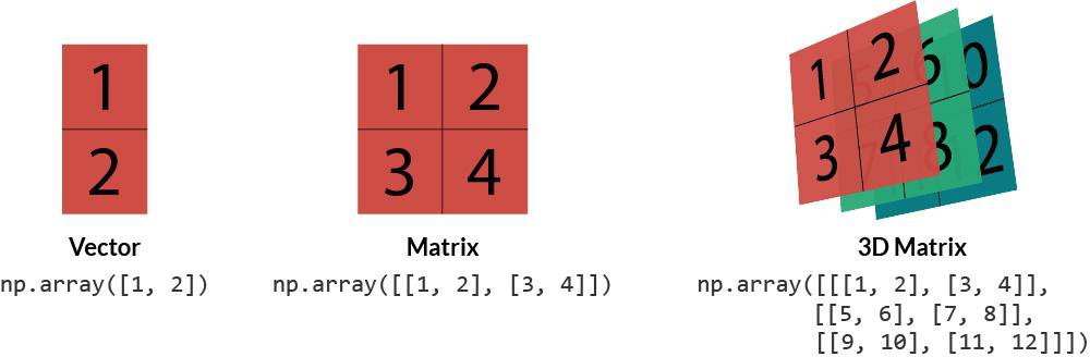
A visual representation of how a vector, a matrix, and a 3D matrix can be created using NumPy. A 2D vector is a 1D NumPy array with two elements.
A Practical Example: The GameObject
Let's see this in action with a simple, practical code example. The following resource provides a minimal class for a "game object" that has position and velocity. This is a perfect, stripped-down model for any object moving in a 2D space, including our rocket.
Vectors in Python – Basics and Use Cases - MangoHost
This article provides several use-cases for vectors in Python. We will focus on the physics simulation example.
In the article, find the subsection titled "Game Development and Physics". Read through the GameObject class definition and the update method. Pay close attention to how the position, velocity, and acceleration attributes are initialized and manipulated as NumPy arrays.
Let's break down the key lines from that example:
# In the __init__ method:
self.position = np.array(position, dtype=float)
self.velocity = np.array(velocity, dtype=float)
self.acceleration = np.array([0.0, -9.81]) # gravity

# In the update method:
self.velocity += self.acceleration * dt
self.position += self.velocity * dt
This elegantly demonstrates our learning outcome. Position, velocity, and acceleration are all stored as NumPy arrays. The physics update logic velocity = velocity + acceleration * time_step is translated directly into self.velocity += self.acceleration * dt. This is a vector addition, performed element-wise, just as you learned in the previous lesson. It's concise, readable, and computationally efficient.
In a Rocket Simulation Context
The GameObject example is great for understanding the principle. Now, let's see how the exact same concept applies in a more complex rocket simulation script. The following resource is a post by an engineer who built a 2D rocket simulation. We'll examine snippets of the code to see how vectors are handled.
First, let's see how the initial state of the rocket is defined.
Modeling a Thrust Vector Control Rocket in Python - Nam's Journal
This journal post walks through building a 2D rocket simulator. We will look at how the core state variables are defined.
Find the section "Implementing the 3DOF function". In the second block of code, notice how the initial position and velocity are assigned. The author receives a Python list pos0 and immediately converts it to a NumPy array. A velocity vector is then created from the initial u and w components. Note that in aerospace, it's common to use x for the forward/downrange axis and z for the vertical axis. Focus on these lines showing the creation of position and velocity vectors. Further down, inside the loop that stores results, you can see how the acceleration vector for each time step is stored: np.array([ax, az]). This confirms that force (and thus acceleration) is also being treated as a vector.
This code structure is more complex than the GameObject class, but the underlying principle is identical: pos and vel are NumPy arrays representing 2D vectors.
Now, let's look at how a force vector is calculated. A rocket's thrust is a force. If the engine is gimbaled (angled), that force is split between the vertical (z) and horizontal (x) axes.
Modeling a Thrust Vector Control Rocket in Python - Nam's Journal
Continuing in the same article, let's see how forces are calculated.
Find the section "Making the simulation". A few code blocks down, you will see the calculations for Fx and Fz. Read the code and the explanation that follows. The author uses trigonometry to resolve the total thrust_profile into its x and z components. See these lines where the force vector components are calculated.
This is a fantastic real-world example that ties everything together. The code takes a scalar value for total thrust (peak_thrust) and an angle (gimbal_angle) and uses np.sin and np.cos to calculate the components of the force vector, Fx and Fz. Because thrust_profile is a NumPy array representing thrust over time, Fx and Fz also become arrays. This single block of code calculates the force vector for every point in time during the simulation, using the element-wise operations you're now familiar with.
Conclusion
In this lesson, you've made a critical connection between physics and code. You now have a robust method for representing vector quantities, which are the language of motion in our simulations.
Here are the key takeaways:
- Physical quantities with magnitude and direction (like position, velocity, and force) are called vectors.
- In Python, a 2D vector is conveniently represented by a NumPy array of length 2, where the elements correspond to the x and y components.
- The element-wise arithmetic you learned previously allows for clean and efficient vector arithmetic. For example,
position += velocity * dtupdates the position vector based on the velocity vector. - We can calculate the components of a vector, like force, from its magnitude and direction using trigonometry (
np.sin,np.cos) and apply these calculations to entire time-series arrays.
You now know how to create and represent vectors. But how do we get information back out of them? For instance, how do we calculate the rocket's total speed from its [vx, vy] velocity vector? How do we find the angle of its trajectory? That's precisely what we'll cover in the next lesson, where we'll learn to compute the magnitude and direction of our NumPy vectors.