In our last lesson, you learned how to create NumPy arrays, the foundational data structures for our flight simulator. We focused on creating arrays from lists and, more importantly, generating evenly spaced time arrays with np.linspace. Now that we can create these structures, it's time to put them to work.
This lesson dives into the core of how simulations compute change: performing element-wise arithmetic operations. You will learn how to apply mathematical operations like addition, multiplication, and division to entire arrays at once, a technique that is both powerful and efficient. This is the key to updating the state of our rocket—calculating its new position from its velocity, or its new velocity from its acceleration—across many points in time simultaneously.
The "Engine" of Simulation: Element-Wise Operations
Imagine you have a time array representing the first 10 seconds of a rocket's flight, with a data point every 0.1 seconds.
import numpy as np
time = np.linspace(0, 10, 101)
If the rocket travels at a constant velocity of 50 m/s, how would you calculate its position at every one of those 101 time points? In standard Python, you'd likely use a for loop to iterate through the time list and calculate the position for each point.
NumPy allows for a much more direct approach. You can perform the calculation on the entire array in a single line of code:
velocity = 50
position = velocity * time
This is an element-wise operation. NumPy applies the multiplication by velocity to every single element in the time array, producing a new array, position, of the same size. This isn't just cleaner to write; because NumPy's operations are implemented in highly optimized, low-level code (C/C++), it is dramatically faster than a Python loop, especially for the large arrays we'll be using in our simulations.
Let's explore this concept further through the official NumPy documentation.
NumPy: the absolute basics for beginners#
This document provides a clear, foundational overview of NumPy's capabilities. We'll focus on the section that details basic arithmetic.
Please read the section titled "Basic array operations". It starts by creating two simple arrays, data and ones. Pay close attention to the examples showing element-wise addition, subtraction, multiplication, and division. Notice how the operators (+, -, *, /) work directly on the arrays.
Operations Between Arrays
As you just read, operations can be performed not just between an array and a single number (a scalar), but also between two arrays of the same size. For instance, if you have an array representing an object's velocity at different times and another array representing the time intervals, you can calculate the distance traveled in each interval.
The operation is performed element by element: the first element of the first array is multiplied by the first element of the second array, the second by the second, and so on.

Broadcasting: A Glimpse of NumPy's Magic
What's happening when we execute velocity * time, where velocity is a single number and time is an array? This is an example of a powerful NumPy feature called broadcasting. In simple terms, NumPy "stretches" or "duplicates" the scalar value so that it can be applied to every element of the array.
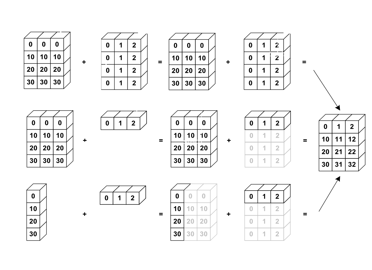
For our purposes, the most important rule of broadcasting is that operations between an array and a single scalar value are always valid. This is fundamental for applying physical constants (like gravity) or conversion factors to an entire dataset at once.
The following video provides a concise, practical demonstration of these concepts, tailored for a technical audience like yourself.
NumPy Tutorial: For Physicists, Engineers, and Mathematicians
This video by Mr. P Solver, aimed at physicists and engineers, quickly demonstrates the power of array operations.
First, watch the segment on basic operations from this timestamp. It perfectly summarizes how a single operation is applied element-wise. Next, watch the segment showing how this is used for plotting from this timestamp. This is a great example of what we'll be doing constantly: creating a linspace array for our x-axis (like time) and then using an element-wise operation (like x**2) to compute the y-values for our plot.
Your Turn: Modeling a Physical System
Now, let's apply these concepts to a concrete physics problem. This will bridge the gap between abstract operations and our goal of simulating motion.
We will use a problem from a computational physics guide.
Tutorial, Part 5: NumPy, SciPy, and Matplotlib - Computational Physics
This tutorial from the University of Toronto provides a hands-on physics problem that is perfect for practicing element-wise operations.
Find "Activity 2" in the text. Read the problem description carefully: it describes an object falling under gravity with air resistance. The velocity v(t) is given by a formula. You are also given the analytical formulas for acceleration a(t) and position x(t), which are the derivative and integral of v(t) respectively. Your task is to use NumPy to calculate and see the values for t, v(t), a(t), and x(t) for the first 20 seconds, at half-second intervals. Don't worry about the calculus for now; just focus on translating the given mathematical formulas into NumPy code. Here's a plan to follow: Define the constants given: terminal speed s_t = 50 m/s and time constant \tau = 5 s. Create a time array t from 0 to 20 seconds with a step of 0.5s. np.linspace or np.arange will work. Translate the formula for velocity v(t) = -s_t (1 - e^{-t/\tau}) into a line of NumPy code. This will use your t array. Note that the exponential function in NumPy is np.exp(). Translate the formulas for acceleration a(t) = -\frac{s_t}{\tau} e^{-t/\tau} and position x(t) = -s_t (t + \tau e^{-t/\tau} - \tau) into NumPy code. Try to write the Python script to do this yourself. Once you're done, you can check your work against the solution in the details block below.
Solution
import numpy as np


# 1. Define constants
s_t = 50.0  # Terminal speed (m/s)
tau = 5.0   # Time constant (s)


# 2. Create the time array
# We need points from 0 to 20, every 0.5s. That's 41 points.
t = np.linspace(0, 20, 41)


# 3. Calculate velocity
# v(t) = -s_t * (1 - exp(-t/tau))
v = -s_t * (1 - np.exp(-t / tau))


# 4. Calculate acceleration and position
# a(t) = (-s_t / tau) * exp(-t/tau)
a = (-s_t / tau) * np.exp(-t / tau)


# x(t) = -s_t * (t + tau * exp(-t/tau) - tau)
x = -s_t * (t + tau * np.exp(-t / tau) - tau)


# Let's print the first 5 values for each to check
print("Time (s):")
print(t[:5])
print("\nPosition (m):")
print(x[:5])
print("\nVelocity (m/s):")
print(v[:5])
print("\nAcceleration (m/s^2):")
print(a[:5])


# The first few position values should be 0, -2.38, -8.96, etc.
# The first few velocity values should be 0, -4.75, -9.05, etc.
# The first few acceleration values should be -10, -9.04, -8.18, etc.
This exercise is a miniature version of what we will do in our full rocket simulation. We start with a time array, then use physical formulas to compute arrays for position, velocity, and acceleration at each of those time points—all without writing a single for loop.
Conclusion
In this lesson, you've added a critical tool to your scientific computing arsenal. You now understand how to perform calculations on entire arrays of data at once, which is the key to efficient simulation.
Here are the main takeaways:
- Element-wise operations allow you to apply arithmetic operators (
+,-,*,/) to every element of a NumPy array simultaneously. - This approach is significantly faster and more readable than using Python
forloops for numerical calculations. - Broadcasting is the mechanism that allows NumPy to perform operations between arrays of different (but compatible) shapes, most commonly an array and a scalar.
- You can translate complex physical formulas directly into NumPy expressions to model how quantities change over time.
You now know how to create arrays and how to perform calculations with them. In the next lesson, we will combine these skills to represent 2D vectors. This will allow us to describe quantities like position and velocity not just as single numbers, but as objects with both magnitude and direction, bringing us one step closer to simulating 2D rocket motion.