Creating NumPy Arrays

Why Do We Need NumPy?

You're already proficient with Python's fundamental data structures like lists. So, why introduce a new one? For scientific computing, efficiency is paramount. A simulation might involve thousands of data points, and we'll need to perform mathematical operations on all of them simultaneously. A standard Python list is a collection of pointers to objects, which makes it flexible but slow for bulk mathematical operations.

NumPy's core object, the ndarray (n-dimensional array), is a grid of values of the same type, stored in a contiguous block of memory. This homogeneity allows NumPy to use highly optimized, pre-compiled C code for its operations, making it orders of magnitude faster than performing the same calculations with Python loops on lists.

For our goal of building a flight simulator, this performance is not just a convenience—it's a necessity.

Creating Arrays from Python Lists

The most straightforward way to create a NumPy array is to convert an existing Python list. The convention for importing NumPy is:

import numpy as np

We then use the np.array() function. For instance, a simple list of numbers becomes a 1D array, which we can think of as a vector. A list of lists becomes a 2D array, or a matrix.

The following image illustrates how Python lists containing numbers are transformed into different dimensional NumPy arrays.

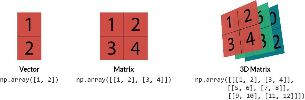
To see why this is so much better for numerical tasks, let's explore a resource that directly compares working with Python lists to NumPy arrays.

As you saw, all elements in a NumPy array must have the same data type, or dtype. When you create an array from a list of integers, NumPy typically creates an array of type int64. If your list contains even one floating-point number, NumPy will promote the entire array to a float type, like float64, to maintain homogeneity. This is crucial because it allows the data to be stored compactly, which is the secret to NumPy's speed.

Generating Arrays with Functions

Often, we don't start with a list of data; instead, we need to generate a sequence of numbers to work with. For example, to simulate a rocket's flight over 30 seconds, we might want to calculate its state at every tenth of a second. Manually creating a list of [0.0, 0.1, 0.2, ...] would be tedious.

NumPy provides functions for this purpose, and one of the most important for simulation is np.linspace.

Linearly Spaced Values with np.linspace

The np.linspace() function creates an array of evenly spaced numbers over a specified interval. Its main arguments are:

1. start: The starting value of the sequence.
2. stop: The final value of the sequence. This value is included in the array.
3. num: The total number of points to generate.

For example, np.linspace(0, 10, 5) will generate 5 evenly spaced values starting at 0 and ending at 10.

This function is incredibly useful for creating time arrays for our simulations or for generating coordinates for plotting.

The following video provides a clear, practical explanation of np.linspace and another related function, np.arange.

So, if we want to simulate the first 60 seconds of a rocket launch with a time step of 0.1 seconds, we would need 601 points (including t=0). We could create the time array like this:

time = np.linspace(0, 60, 601)

This simple line of code gives us a complete, accurate time axis for our entire simulation, ready for the next steps.

Your Turn: Create Some Arrays

Let's put this into practice. Open a Python environment (like a Jupyter notebook or a simple script) and try the following:

1. First, make sure you have NumPy imported: import numpy as np.
2. Create a NumPy array named force_values from the following Python list, which could represent force measurements in Newtons: [100.5, 99.8, 99.7, 101.0, 100.2].
3. Imagine you need to model the first 10 seconds of a rocket motor burn. Create a time array named burn_time that contains 100 evenly spaced points from t=0 to t=10.
4. Print both arrays and observe their structure.

import numpy as np




# 1. Create array from a list
force_data = [100.5, 99.8, 99.7, 101.0, 100.2]
force_values = np.array(force_data)
print("Force values:")
print(force_values)
print(f"Data type: {force_values.dtype}\n") # Should be float64




# 2. Create a time array using linspace
burn_time = np.linspace(0, 10, 100)
print("Burn time array (first 10 values):")
print(burn_time[:10]) # Print just the first 10 for brevity
print(f"Total elements: {len(burn_time)}") # Should be 100

Conclusion

In this lesson, you took the first crucial step in our journey toward flight simulation. You've learned how to create the fundamental data object we will be using throughout this course: the NumPy array.

Here are the key takeaways:

• NumPy arrays are the high-performance data structure for numerical and scientific computing in Python. Their efficiency comes from storing data of a single type (dtype) in a contiguous block of memory.
• You can create an array directly from a Python list using np.array(). This is useful when you have pre-existing data.
• You can generate an array of evenly spaced numbers using np.linspace(start, stop, num). This is ideal for creating sequences like time steps or spatial coordinates for our simulations.

Now that you know how to create these arrays, the next logical step is to learn how to perform calculations with them. In our next lesson, we will cover element-wise arithmetic operations. This will unlock our ability to update the state of our simulation—for example, calculating a new position based on a velocity, which is the heart of simulating motion.