Introduction
Welcome to the next lesson on our path to process optimization. In the previous session, you successfully built and validated a second-order process model from your Response Surface Methodology (RSM) experiment data. You now have a reliable regression equation that describes the relationship between your process inputs (factors) and the key output (response). This equation is the foundation for optimization.
This lesson directly addresses our learning outcome: Use contour plots and optimization tools to identify optimal process settings from a response surface model. Now that we have the map (our model), we will learn how to read it to find the treasure—the specific combination of factor settings that gives us the best possible process performance. We'll explore two key approaches:
- Visualizing the surface using contour and 3D surface plots to intuitively understand the process landscape.
- Using numerical optimizers to pinpoint the exact optimal settings, especially when balancing multiple competing objectives.
1. Visualizing the Process Landscape
The second-order model you built is a mathematical representation of a multi-dimensional surface. To understand it, we need to visualize it. The two most common tools for this are the 3D surface plot and the contour plot.
- 3D Surface Plot: This plot provides a three-dimensional view of the response surface, showing how two factors at a time affect the response. It's great for getting an intuitive feel for the shape of the surface—whether it has peaks, valleys, or ridges.
- Contour Plot: This is a two-dimensional, top-down view of the same surface, much like a topographical map. Lines on the plot connect points of equal response value. The closer the lines, the steeper the "slope." Colors often indicate the "elevation" (response value), helping you quickly spot high- and low-performing regions.
Let's watch a practical demonstration of how to generate and interpret a contour plot for a single response.
Response Surface Methodology Box Behnken Design in MINITAB | RSM Box Behnken Optimization
This video from 'Engineering and Info' demonstrates how to create a contour plot in Minitab for a machining process. The goal is to maximize the material removal rate (MRR).
Please watch from 04:42 to 06:26. Focus on how the presenter interprets the colors and lines on the contour plot to identify the region where the material removal rate is highest. Notice how they can swap factors on the axes to explore different relationships.
As you saw, contour plots allow you to visually identify an "operating window" where your process is likely to perform well. For a simple case with only two factors, you might even be able to pick your optimal settings right from this plot. However, with more factors or more complex surfaces, we need a more precise tool.
2. Numerical Optimization for a Single Response
Visual plots give you the general location of the optimum, but statistical software can calculate the precise settings for you using a response optimizer. This tool uses the regression model you built to find the factor settings that achieve a specific goal:
- Maximize the response (e.g., yield, strength)
- Minimize the response (e.g., defects, impurities, cost)
- Target a specific value (e.g., viscosity, coating thickness)
The optimizer evaluates how well any given combination of settings meets your goal and assigns it a Desirability score from 0 (completely undesirable) to 1 (perfectly meets the goal). It then finds the settings that result in the highest desirability.
Let's see this in action.
Response Surface Methodology Box Behnken Design in MINITAB | RSM Box Behnken Optimization
Continuing with the same machining example, the video now demonstrates how to use Minitab's Response Optimizer.
Please watch from 07:03 to 08:34. Pay close attention to: Setting the Goal: How the goal for the response (maximize MRR) is specified. The Optimizer Output: How the tool displays the optimal factor settings (cutting speed, feed rate, depth of cut) and the predicted response at those settings. The Desirability Score: Note the composite desirability value and how a value close to 1 indicates a highly desirable outcome.
This optimizer is an incredibly powerful tool. You input the goal, and it gives you the recipe for achieving it. But what happens when you have more than one recipe to follow at the same time?
3. The Real-World Challenge: Optimizing Multiple Responses
In nearly any real manufacturing process, you have to balance competing priorities. You might want to maximize production rate, but you must also minimize defect levels and control costs. This is where multi-response optimization becomes essential—a key skill for a Black Belt.
Often, these goals are contradictory. The settings that maximize yield might also produce unacceptable levels of an impurity. The challenge is to find a compromise—a "sweet spot" that produces the best overall outcome across all responses.
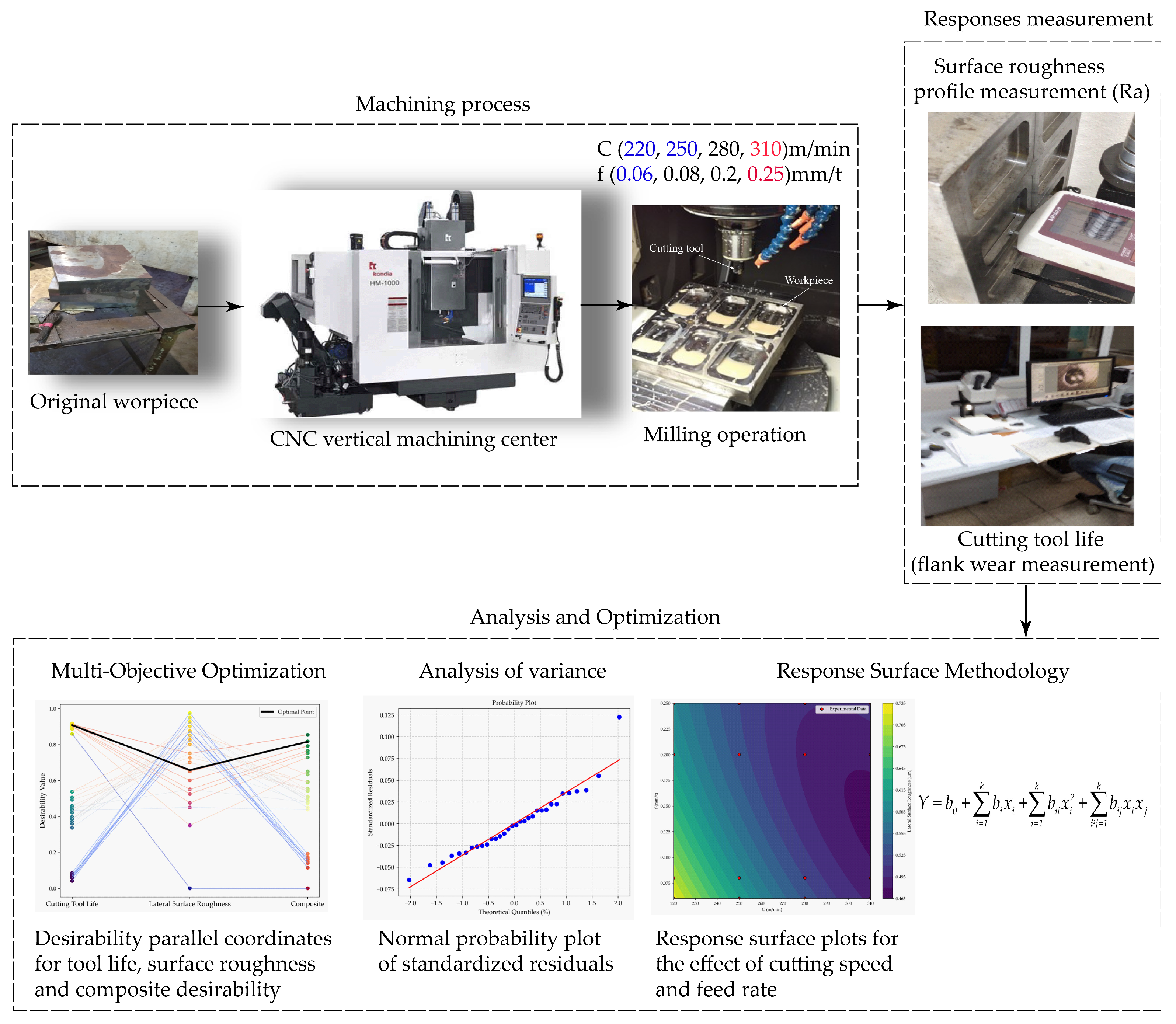
To do this, we extend the concept of desirability. The software calculates an individual desirability score (0 to 1) for each response. Then, it combines these into a single composite desirability score, which represents the overall "goodness" of a particular outcome.
Temperature Optimization by Using Response Surface Methodology ...
This research paper on optimizing a machining process provides a good, practical explanation of the concept behind this technique, known as Desirability Function Analysis (DFA).
Please read section 3.2. Implementation of DFA. Don't worry about memorizing the equations. Focus on understanding the logic: how an individual desirability score (di) is calculated for a response, and how these are combined into a Composite Desirability (CD) using a geometric mean (Equation 5). Then, skim through the figures in the following section (Figures 6-12) to see how contour and surface plots can be generated for the desirability itself, helping you visualize the regions that offer the best compromise.
Now let's see how this is applied to find a workable solution when faced with conflicting goals.
Using Overlaid Contour Plots
One of the best visual tools for multi-response optimization is the overlaid contour plot. This plot draws the contour lines for each response on a single graph. You define the acceptable range for each response (e.g., "Yield > 80%" and "Impurity < 0.5%"), and the plot shades the area where all conditions are met simultaneously. This shaded region is your feasible operating window.
Multiple Response Optimization Explained with Example using Minitab Response Surface Methodology RSM
This video from 'The Open Educator' provides a fantastic walkthrough of optimizing a process with two competing responses: maximizing yield while targeting a specific viscosity.
Please watch the video from the beginning to 06:19. The key segments are: The Problem (0:00 - 1:34): Understand the contradictory nature of the two responses. Creating the Overlaid Plot (2:44 - 3:50): See how the acceptable ranges for both yield and viscosity are defined. Interpreting the Plot (3:50 - 5:07): Focus on how to identify the white, unshaded area—the sweet spot that satisfies both criteria. Using the Optimizer (5:07 - 6:19): Observe how the response optimizer is used to find the single best setting within that sweet spot.
Making the Final Decision
The overlaid contour plot shows you the feasible region, and the response optimizer gives you the mathematically "best" point within it. In practice, as an engineer, you would use this information to make an informed decision. Sometimes, the mathematically optimal point might be at the very edge of the feasible region, which could be risky if the process drifts. You might choose a more robust point in the center of the window.
The NIST handbook example, which you looked at briefly in the last lesson, illustrates this decision-making process.
Response surface model example
Let's revisit the NIST example. After building separate models for 'Uniformity' and 'Stress', the engineers needed to find a single setting for both.
Please read the final two sections of the article: 'Response Surface Contours for Both Responses' and 'Summary'. Note how the engineers recognized the trade-off (high pressure is good for one response, bad for the other) and used their process knowledge to make a final, pragmatic decision.
This final step of applying process knowledge to the statistical output is what separates a good analyst from a great one. The tools give you the optimal solution based on the data, and your expertise helps you confirm and implement it effectively.
Conclusion
In this lesson, you have moved from a validated mathematical model to actionable process settings. This is the ultimate goal of the "Improve" phase in a DMAIC project.
Key Takeaways:
- Contour plots and 3D surface plots are essential tools for visualizing your process model and identifying promising operating regions.
- The Response Optimizer provides a precise, numerical solution by finding the factor settings that maximize, minimize, or hit a target for your response(s).
- The concept of Desirability (from 0 to 1) is used to score how well a given setting meets your goals.
- For multiple, often conflicting, responses, a composite desirability score is calculated. You can find the optimal compromise using the optimizer and visualize the feasible operating window with overlaid contour plots.
Preview of the Next Lesson:
You have now identified the proposed optimal settings for your process. But before you roll out the changes across the factory floor, a few crucial steps remain. In our next lessons, we will cover how to evaluate and select proposed solutions using a Pugh matrix (if you have multiple competing solutions) and how to proactively manage risks of the new process settings by conducting a Failure Mode and Effects Analysis (FMEA). This ensures your optimized solution is not only effective but also robust and safe.