Introduction
Welcome to your next lesson in the "Quantifying Process Performance" module. In our last session, we focused on establishing a process baseline. You learned how to use historical data to calculate key metrics like yield and Parts Per Million (PPM), creating a clear "before" snapshot of your process. This baseline is the quantitative foundation for any DMAIC project.
As we previewed, many of the most powerful statistical tools in Six Sigma, such as process capability analysis (Cp/Cpk) and hypothesis testing, operate on the assumption that your data follows a normal distribution—the classic "bell curve." Using these tools on data that isn't normal can lead to flawed conclusions.
Therefore, this lesson is dedicated to the learning outcome: Assess normality of process data using probability plots and statistical tests (e.g., Anderson-Darling). We will explore why this assumption is critical and learn the practical methods, both graphical and statistical, to verify it before proceeding with further analysis.
1. Why is Normality Important?
The normal distribution is a specific, symmetrical, bell-shaped distribution that serves as a foundation for a vast range of statistical methods. When your data is normally distributed, we can make reliable predictions about its behavior.
Many statistical procedures you'll encounter in your Green and Black Belt journey—including t-tests, ANOVA, and, most pressingly for us, process capability analysis—are built on this assumption. If we analyze non-normal data as if it were normal, our calculations for process capability (like Cpk) and defect rates will be inaccurate, potentially leading us to misjudge process performance and make poor decisions.
To understand the basics of normality and the two primary ways to test for it, please watch the first minute of this video.
Normality test [Simply Explained]
The video 'Normality test [Simply Explained]' from numiqo provides a concise overview of why normal distribution matters for hypothesis testing and introduces the two main assessment approaches: analytical (statistical tests) and graphical (plots).
Watch the video from the beginning to the 01:01 mark to get a foundational understanding of the concept.
As the video states, we have two complementary methods for checking normality: analytical tests that provide a statistical conclusion, and graphical plots that provide visual context. A robust assessment always uses both.
2. The Graphical Approach: Probability Plots
The most powerful graphical tool for assessing normality is the Normal Probability Plot (also known as a Quantile-Quantile or QQ Plot).
Instead of a histogram's bars, a probability plot displays your data points against the theoretical values they would have if they came from a perfectly normal distribution.
How to Interpret a Probability Plot:
- If the data is normal: The points will fall closely along a straight, diagonal line.
- If the data is not normal: The points will deviate from the straight line in a systematic pattern (e.g., a curve or an S-shape).
A simple, practical way to evaluate this is the "fat pencil test." If you can imagine laying a fat pencil over the line and covering most of the data points, your data is likely normal enough for practical purposes.
Compare the two plots below.

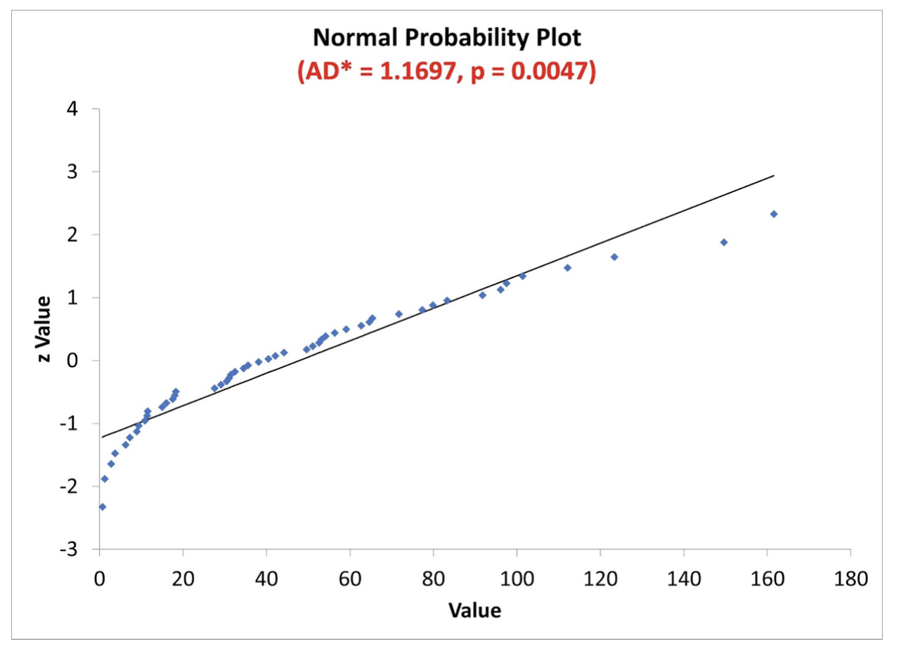
Deviations from the line aren't just random; their patterns can tell you how the data is non-normal. This is incredibly useful for root cause analysis.
A Simple Guide to Probability Plots
The Minitab blog post 'A Simple Guide to Probability Plots' does an excellent job of explaining how to interpret the visual patterns you might see. It moves beyond a simple 'normal vs. non-normal' conclusion.
Please read the article starting from the introduction down to the end of the 'Example: Probability Distribution Plots Using Laser Game Data' section. Focus on how to visually identify: The 'fat pencil' test. Asymmetrical distributions (curved patterns). Discrete data or insufficient measurement resolution (stair-step patterns). Outliers and mixed populations (broken lines or distinct groups of points).
As you can see from the reading, a probability plot is more than just a pass/fail test; it's a diagnostic tool. In a manufacturing setting, seeing multiple "lines" of data might indicate you've mixed products from different machines, shifts, or raw material batches.
3. The Analytical Approach: Statistical Tests
While a probability plot gives you visual context, a statistical test provides a formal, objective conclusion. The process is a form of hypothesis testing.
- Null Hypothesis (H₀): The data is from a normal distribution.
- Alternative Hypothesis (H₁): The data is not from a normal distribution.
The test calculates a p-value, which represents the probability of seeing your data if the null hypothesis were true. The decision rule is:
- If p-value > 0.05: We fail to reject the null hypothesis. We conclude the data is normal.
- If p-value ≤ 0.05: We reject the null hypothesis. We conclude the data is not normal.
(Note: 0.05 is the most common significance level, or alpha, but can be adjusted.)
The following video demonstrates how to perform and interpret the most common normality tests in Minitab, a standard software in Six Sigma.
Normality Test With Example | What Is Normality | Normality Test In Minitab & SigmaXL
The video 'Normality Test With Example' from LEARN & APPLY provides a practical walkthrough. It introduces the three main tests available in Minitab and explains how to interpret the p-value in a manufacturing context.
Please watch from the beginning up to the 07:10 mark. Pay close attention to: The explanation of the null and alternative hypotheses. The description of the three tests: Anderson-Darling, Ryan-Joiner, and Kolmogorov-Smirnov. The step-by-step process in Minitab and, most importantly, the interpretation of the resulting p-value.
Which Statistical Test is Best?
As the video mentioned, Minitab and other software offer several tests. While Anderson-Darling (A-D) is the default and a great all-around choice, there are nuances that are important at the Black Belt level.
- Anderson-Darling (A-D): This test is particularly sensitive to differences in the tails of the distribution. This is highly relevant in manufacturing, as out-of-spec parts are often found in the tails. It is very effective at detecting shifts in a process.
- Ryan-Joiner (R-J): This test is based on correlation and is particularly powerful at detecting the presence of one or two large outliers.
- Kolmogorov-Smirnov (K-S): Generally less powerful than the other two for detecting non-normality and is less commonly used as the primary test in quality improvement projects.
For a deeper dive into choosing the right test for a specific manufacturing scenario, this brief article is highly informative.
Anderson-Darling, Ryan-Joiner, or Kolmogorov-Smirnov - Minitab Blog
This Minitab blog post, 'Anderson-Darling, Ryan-Joiner, or Kolmogorov-Smirnov,' compares the tests using simulated manufacturing data.
Read the introduction and the sections describing the three scenarios (outliers, process shifts). Then read the 'In summary' section at the end. Focus on the conclusion about when to use the Ryan-Joiner test (if you suspect outliers) versus the Anderson-Darling test (if you suspect process shifts).
The key takeaway is that for general-purpose use, Anderson-Darling is an excellent default. However, if your process knowledge suggests that sporadic outliers are the main issue, the Ryan-Joiner test might be more effective.
Putting It All Together: A Robust Workflow
Neither the graphical plot nor the statistical test tells the whole story on its own. A large dataset might produce a statistically significant p-value (p < 0.05) even if the probability plot shows only a minor, practically irrelevant deviation from normality. Conversely, a small dataset might have a high p-value even with a visually suspect plot.
Therefore, the best practice is to combine both:
- Generate a Normal Probability Plot with an accompanying Anderson-Darling test.
- Examine the plot visually. Does it pass the "fat pencil test"? Are there any obvious patterns like curves, steps, or outliers that might indicate a special cause or a different underlying distribution?
- Check the p-value. Is it greater than the significance level (typically 0.05)?
- Synthesize the findings.
- Plot looks good AND p > 0.05: Your data is normal. Proceed with your analysis.
- Plot looks bad AND p ≤ 0.05: Your data is not normal. You must address this before proceeding.
- Mixed signals (e.g., plot looks okay but p ≤ 0.05): This often happens with very large datasets. Use your process knowledge. If the deviation from the line is minor, you may be able to treat the data as "practically" normal. If you're unsure, it's safer to assume it's non-normal.
Conclusion
In this lesson, you have learned the critical importance of checking your data for normality before applying many common statistical tools. You are now equipped to perform this assessment using the two essential methods: graphical analysis with probability plots and analytical confirmation with statistical tests like the Anderson-Darling test.
Key Takeaways:
- Normality is a key assumption for many statistical tools, including process capability analysis (Cp/Cpk).
- Always use a two-pronged approach: a graphical plot for visual context and a statistical test for an objective conclusion.
- A Normal Probability Plot should show points falling along a straight line. Patterns in deviations can provide diagnostic clues about your process.
- For a normality test, the null hypothesis is that the data is normal. A p-value greater than 0.05 typically supports this assumption.
- The Anderson-Darling test is a powerful, all-purpose choice for normality testing in manufacturing contexts.
Preview of the Next Lesson:
This naturally leads to the question: "What do I do if my data isn't normal?" You don't just stop your project. In the next lesson, we will address this by learning how to apply a Box-Cox transformation to non-normal data to enable valid capability analysis. This powerful technique allows us to mathematically alter the data so it becomes normal, unlocking the use of all the standard statistical tools you're learning.