Establishing Process Baselines from Historical Data

1. What is a Process Baseline?

Before you can improve a process, you must first understand its current state in measurable terms. This is the purpose of establishing a process baseline. It's a quantitative starting point against which all future improvements will be measured.

It's important to distinguish baselining from benchmarking:

• Baselining is inward-looking. It measures the current capability of your process.
• Benchmarking is outward-looking. It compares your process performance against competitors or best-in-class examples.

In a Six Sigma project, you always start with baselining. To learn more about this concept, please read the introductory sections of the following guide.

As the reading highlights, baselining uses available historical data to get a quick but data-driven estimate of your key processes' performance. This allows you to identify which processes have the most significant improvement opportunities.

2. Key Baseline Metrics

To quantify performance, we use a set of standardized metrics. These allow us to describe process performance in a common language. The most common baseline metrics are derived from defect data.

Metrics from Discrete (Attribute) Data:

• Defects Per Unit (DPU): The average number of defects found per unit inspected.
  • Formula: Total Defects / Total Units
• Defects Per Million Opportunities (DPMO): A more refined metric that accounts for the fact that a single unit can have multiple opportunities for a defect. This is a cornerstone metric in Six Sigma.
  • Formula: (Total Defects / (Total Units × Opportunities per Unit)) × 1,000,000
• Yield: The percentage of units that pass inspection without any defects. First Pass Yield (FPY) is the most common measure.
  • Formula: (Total Units - Defective Units) / Total Units
• Sigma Level (Z): A single number that represents the capability of a process, directly converted from its DPMO value. A higher Sigma Level means fewer defects.

The MindPro guide provides a superb, practical example of baselining several manufacturing processes.

Metrics from Continuous Data:

When you have measurement data (e.g., dimensions, temperature, pressure), you can calculate the baseline performance relative to engineering specifications.

• Parts Per Million (PPM) Defective: This is the number of measured parts that fall outside the Lower Specification Limit (LSL) or Upper Specification Limit (USL), scaled to one million.
• Performance Indices (Pp, Ppk): These are long-term capability indices calculated from the overall variation of historical data. They tell you how capable your process has been performing historically. We will cover these in much greater detail in a future lesson.

3. Case Study: Baselining a Fuel Injection Pump Assembly

Now let's see how these concepts are applied in a real DMAIC project. We'll use a case study about improving the assembly of fuel injection pumps, where the initial problem was a low first-pass yield of only 85%.

Let's break down what the team did:

1. Identified the Problem: The first-pass yield was only 85%, and there were significant customer complaints. The Critical-to-Quality (CTQ) characteristic was the clearance between a barrel and plunger.
2. Validated the Measurement System: They performed a Gage R&R study and found it to be acceptable (19.53%), giving them confidence in their data.
3. Collected Baseline Data: They created a data collection plan and gathered 1,361 data points for the clearance value over two weeks.
4. Calculated Baseline Metrics: They analyzed this historical data. As shown in Figure 2 of the paper, the analysis revealed a PPM Total of 157,972. This means for every million assemblies, nearly 158,000 were out of specification. This number became their official process baseline. This DPMO corresponds to the 85% yield mentioned at the start.

The image below shows a similar type of output from a process capability analysis used for baselining. It visualizes the data in a histogram and provides the key performance metrics in a summary table.

4. The Baselining Workflow

Based on the case study and best practices, here is a simple workflow for establishing a process baseline:

1. Define Scope: Clearly identify the process and the critical CTQ(s) you need to measure.
2. Validate Measurement System: Confirm that your measurement system is capable using Gage R&R or Attribute Agreement Analysis. Never baseline with a bad measurement system.
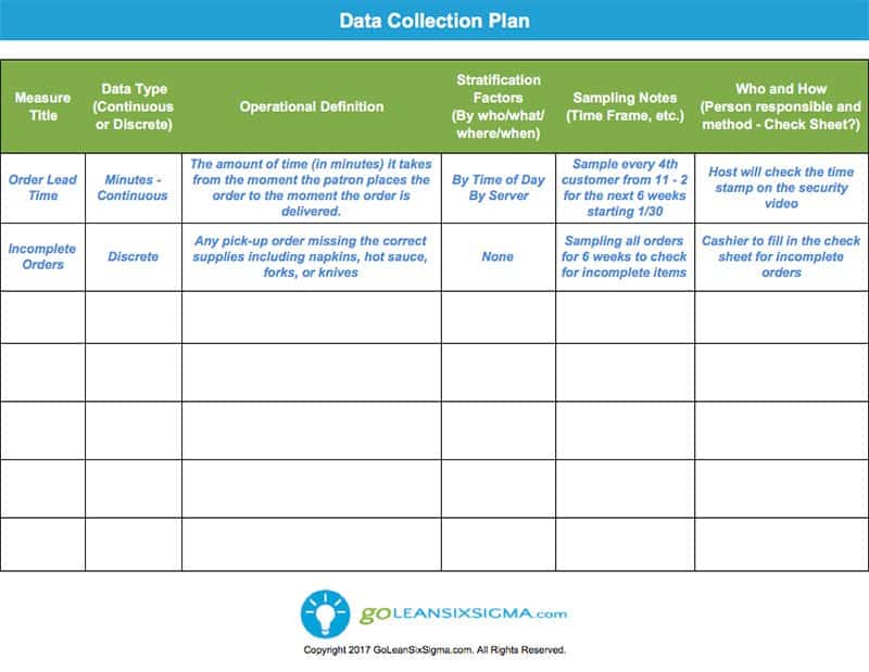
3. Plan & Collect Data: Use a structured Data Collection Plan to gather sufficient historical data (typically at least 30-50 data points, but more is better).

4. Visualize and Analyze: Plot the data in a histogram or run chart to understand its distribution and behavior over time.
5. Calculate & Document: Calculate the key baseline metrics (Yield, DPMO/PPM, Sigma Level) and document this as your project's starting point.

Quick Check-in

Let's test your understanding with a simple manufacturing scenario.

• Scenario: An automated process cuts wires to a specified length. The specification is 100mm ± 2mm. You have inspection data from the last month for 5,000 wires. Your digital measurement system has been validated. The data shows that 75 wires were too short (<98mm) and 50 wires were too long (>102mm).

• Questions:

  1. How many total defects were found?
  2. What is the baseline process yield?
  3. What is the baseline defect rate in Parts Per Million (PPM)?

Answers:

1. Total Defects = 75 (short) + 50 (long) = 125 defects.
2. Yield = (5,000 - 125) / 5,000 = 4,875 / 5,000 = 97.5%.
3. PPM = (125 defects / 5,000 total parts) * 1,000,000 = 25,000 PPM.

This quantified baseline (97.5% yield, 25,000 PPM) is the concrete starting point for any improvement project on this process.

Conclusion

You have now learned how to establish a process baseline, one of the most important deliverables of the Measure phase. By quantifying the current state, you create a clear, objective benchmark for your project. Without a reliable baseline, you can never definitively prove that your improvement efforts have had a meaningful impact.

Key Takeaways:

• A process baseline is a quantitative "before" picture of your process's performance, established using historical data.
• It is crucial to validate your measurement system before you establish your baseline.
• Key baseline metrics for attribute data include Yield, Defects Per Unit (DPU), and Defects Per Million Opportunities (DPMO).
• For continuous data, Parts Per Million (PPM) defective is the primary baseline metric.
• These metrics can be used to calculate an overall Sigma Level for the process.

Preview of the Next Lesson:
When you look at a histogram of your baseline data, you might assume it follows a nice, symmetrical bell curve—the "normal distribution." However, manufacturing data is often not normal. It can be skewed or have other strange shapes. Performing capability analysis on non-normal data as if it were normal can lead to incorrect conclusions.

In our next lesson, we will learn how to assess the normality of process data using probability plots and statistical tests. This is a critical next step before we can conduct a formal and accurate process capability analysis.