Introduction
Welcome back! In our last lesson, we established a crucial step in any data-driven project: assessing whether your process data follows a normal distribution. You learned how to use the powerful combination of graphical probability plots and statistical tests, like the Anderson-Darling test, to make an objective decision.
We concluded by asking the critical question: "What do you do if your data isn't normal?" Many of the most important Six Sigma tools, especially process capability analysis, are invalid for non-normal data. This lesson provides the answer.
Today, we will focus on the learning outcome: Apply a Box-Cox transformation to non-normal data to enable valid capability analysis. You will learn a standard, powerful technique for mathematically transforming non-normal data so that it becomes normal, thereby "unlocking" the full suite of statistical analyses you need to quantify and improve your process.
1. The Problem: When Capability Analysis Fails
Imagine you're leading a project to reduce the lead time for a new product release. The target is to complete the release in 25 days or less. You collect data, run a capability analysis in Minitab, and get the output. But as we learned in the last lesson, the first thing you must check is the normality assumption.
Let's watch a short segment of a video that walks through this exact scenario. It will demonstrate how a standard capability analysis flags the data as non-normal, creating a roadblock.
Process Capability for Non-Normal Distribution Using Minitab-Case study
The video 'Process Capability for Non-Normal Distribution' from Knowledge Factory presents a case study on reducing lead time. This segment will show the initial capability analysis and how the normality test fails.
Watch from 02:27 to 04:32. Focus on: The setup of the capability analysis in Minitab. The interpretation of the control charts (showing stability). The interpretation of the normal probability plot and the p-value, which confirms the data is not normal.
As the video shows, the p-value is less than 0.005, forcing us to reject the null hypothesis. The data is not normal. Therefore, the calculated Cpk and Ppk values on that report are not reliable. We need a way to deal with this non-normality to proceed.
2. The Solution: Data Transformation
When faced with non-normal data, we have a few options. We could try to find a different statistical distribution that fits the data (like Weibull or Lognormal), or we could use non-parametric tests. However, a very common and powerful approach is data transformation.
Data transformation is the process of applying a consistent mathematical function to every data point in your dataset to change the shape of its distribution. The goal is to make the distribution normal so that standard statistical tools can be used.
The following video provides an excellent introduction to this concept.
Data Transformation With Example | Box-Cox Transformation
The video 'Data Transformation With Example' from LEARN & APPLY explains the what, why, and when of data transformation before introducing the Box-Cox method.
Please watch the first 5 minutes and 40 seconds (00:00 to 05:40). Pay attention to: The definition of data transformation. The primary reason for transformation: satisfying the normality assumption for statistical analysis. The options available when data is not normal (including transformation).
The key takeaway is that transformation provides a path forward, allowing us to use familiar and powerful tools like capability analysis even when our raw data doesn't cooperate.
3. How the Box-Cox Transformation Works
One of the most widely used methods in Six Sigma is the Box-Cox transformation. It's a type of power transformation that systematically tests different exponents (referred to by the Greek letter lambda, ) on your data to find which one results in the most "normal" distribution.
Key Characteristics of Box-Cox:
- It is only effective for positive data (values > 0). This is very common for manufacturing data like cycle time, pressure, temperature, or strength measurements.
- It finds an "optimal" that minimizes the standard deviation of the transformed data, which has the effect of making it more normal.
The value of corresponds to a specific mathematical operation:
| Lambda () | Transformation Formula | Common Name |
|---|---|---|
| 2 | Square | |
| 1 | No transformation | |
| 0.5 | Square Root | |
| 0 | Natural Log | |
| -0.5 | Inverse Square Root | |
| -1 | Inverse/Reciprocal | |
| -2 | Inverse Square |
You don't need to perform these calculations by hand. Statistical software like Minitab automates the search for the best . The output is typically a Box-Cox plot.
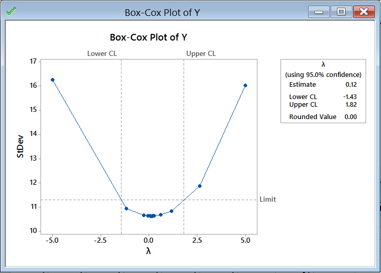
The plot also includes a 95% confidence interval for the optimal . A crucial rule of thumb: If the confidence interval includes , no transformation is necessary. In the plot above, the interval is [-1.43, 1.82], which does include 1, suggesting a transformation might not be strictly required despite the optimal value being near zero. In practice, you combine this with the p-value from your initial normality test to make a final decision.
4. A Practical Walkthrough
Let's walk through the complete process, from identifying non-normal data to performing a valid capability analysis on the transformed data.
The following guide provides an exceptionally clear, step-by-step example based on a manufacturing production run.
The document 'Box-Cox Transformation' from SPC for Excel provides a detailed, practical guide. It covers identifying non-normality, the logic of the transformation, verifying the result, and seeing the impact on Cpk.
Please read this PDF from start to finish. It's a concise and highly relevant document. As you read, focus on this four-step workflow: Confirm Non-Normality (Pages 4-5): Notice how the author uses a histogram and a normal probability plot to conclude the data is not normal (p-value = 0.0131). Find the Optimal Transformation (Pages 6-7): Understand how the software searches for the \lambda that minimizes variation and presents it in the Box-Cox plot. The optimal \lambda is 0.44, which is rounded to 0.5 (a square root transformation). Verify the Transformation (Pages 7-8): This is a critical step. The author creates a new probability plot of the transformed data and confirms it is now normal (p-value = 0.45). Compare the Capability Analysis (Page 9): Look at Figure 8 (invalid analysis on raw data) and Figure 9 (valid analysis on transformed data). The Cpk values are different, but the one from the transformed data is the one you can trust.
To see this workflow in action within Minitab, the following video provides a clear demonstration.
Data Transformation With Example | Box-Cox Transformation
The video 'Data Transformation With Example' that we started earlier also contains a full Minitab demonstration.
Watch the segment from 06:56 to the end (15:57). The presenter follows the same logic as the PDF: He first confirms the data is non-normal (12:00). He performs the Box-Cox transformation (12:55). He interprets the Box-Cox plot, noting the optimal lambda and the confidence interval (14:20). He concludes that a transformation is appropriate and what it should be (inverse transformation, since lambda is rounded to -1).
5. Important Considerations
The Box-Cox transformation is a powerful tool, but it's not a magic bullet. Here are two key points to remember:
-
Limitations: As mentioned, Box-Cox only works for data that is strictly positive (> 0). If your data includes zeros or negative values, you would need to use a more powerful method like the Johnson transformation. This is typically covered in more advanced Black Belt training, but it's good to be aware of it.
-
Transformation vs. Understanding: Transformation fixes the data so you can perform a valid analysis. It does not, however, explain why the data was non-normal in the first place. Is there a natural process boundary? Are you mixing data from different shifts or machines? Always use your process knowledge to investigate the root cause of non-normality. Transformation is a statistical tool, not a substitute for process investigation.
As the research paper below notes, transformation is one of two main approaches. The other is to find an alternative distribution that fits your data without changing it. For a Green Belt, mastering the Box-Cox transformation is the primary requirement.
Assessment of process stability and capability in a manufacturing ...
The research paper 'Assessment of process stability and capability' reinforces the concepts we've learned in a real-world case study.
Quickly read the introduction on page 2 and review the figures on pages 6-7. Notice how the authors identify non-normal data (Figure 9, p-value=0.039), apply a Box-Cox transformation (Figure 11), and then re-check the transformed data for normality (Figure 12, p-value > 0.05). This concisely shows the exact workflow we've been studying.
Conclusion
In this lesson, you've added a vital tool to your Six Sigma toolkit. When faced with the common problem of non-normal data, you now have a standard, reliable method to overcome it.
Key Takeaways:
- Process capability analysis (Cp/Cpk) is not valid for non-normal data.
- The Box-Cox transformation is a power transformation used to make non-normal, positive data fit a normal distribution.
- The transformation is defined by a parameter, lambda (), which statistical software finds by minimizing the variation in the transformed data.
- Always verify that the transformation was successful by running a normality test on the new, transformed data before proceeding with capability analysis.
- Transformation enables valid statistical analysis, but you should still investigate the underlying process reasons for non-normality.
Preview of the Next Lesson:
Now that we have established how to properly handle both normal and non-normal data, we are ready to dive deep into the metrics themselves. In our next lesson, you will learn to calculate and interpret Cp, Cpk, Pp, and Ppk indices to assess process capability against specifications. We will break down what each of these indices tells you about your process and how they differ from one another.