Chi-Square Tests for Attribute Data Analysis

Understanding the Chi-Square Test

At its core, the Chi-Square (${\chi }^2$) test is designed to analyze categorical data. It works by comparing the actual counts you observed in your sample (the Observed frequencies) with the counts you would expect to see if there were no relationship at all between the variables (the Expected frequencies).

If the observed counts are very different from the expected counts, the Chi-Square statistic will be large, leading to a small p-value. This indicates that the difference is unlikely to be due to random chance, and we can conclude that a significant relationship exists.

There are a couple of types of Chi-Square tests, but for our purposes of comparing two categorical factors, we will focus on the Chi-Square Test of Independence.

Applying the Chi-Square Test of Independence: A Step-by-Step Example

The best way to understand the Chi-Square test is to apply it to a practical manufacturing scenario. We'll use the example from the article you just reviewed, which is highly relevant to your work.

Scenario: A manufacturing team wants to know if the type of defect that occurs is independent of the production shift ('Day' vs. 'Night'). They collect data on 60 defects, categorizing them by type and shift.

The data is organized into a contingency table, which is the standard format for a Chi-Square analysis.

Now, let's walk through the formal hypothesis testing procedure.

Step 1: State the Hypotheses

As with all hypothesis tests, we start with a null and an alternative hypothesis. For a test of independence, they are always framed as:

• Null Hypothesis (H₀): The two variables are independent.
  • In our example: Defect type is independent of the production shift.
• Alternative Hypothesis (H₁): The two variables are not independent (they are associated).
  • In our example: Defect type is associated with the production shift.

Our goal is to see if we have enough evidence to reject the null hypothesis in favor of the alternative. We'll use a standard significance level of $\alpha =0.05$.

Step 2: Calculate the Expected Frequencies

This is the most critical step. We need to calculate what the counts in each cell of our contingency table would be if the null hypothesis of independence were true.

The formula for the expected count (E) in any cell is:
$E=\frac{(\text{Row Total})\times (\text{Column Total})}{\text{Grand Total}}$

The intuition is that if the variables are independent, the proportion of each defect type should be the same for both shifts.

Let's watch a video that provides an excellent walkthrough of this calculation and the logic behind it.

Step 3: Calculate the Chi-Square Statistic (${\chi }^2$)

The ${\chi }^2$ statistic measures the total discrepancy between the observed (O) and expected (E) counts across all cells in the table.

The formula is:
${\chi }^2=\sum \frac{(O-E{)}^2}{E}$

You calculate $\frac{(O-E{)}^2}{E}$ for each cell and then sum them all up. A larger ${\chi }^2$ value indicates a greater difference between your data and what you'd expect under independence.

Step 4: Determine Degrees of Freedom and Find the P-value

• Degrees of Freedom (df): This determines the shape of the Chi-Square distribution we compare our statistic against. For a test of independence, the formula is simple:
  $\text{df}=(\text{Number of Rows}-1)\times (\text{Number of Columns}-1)$
  For our 2x3 table (2 shifts, 3 defect types), df = (2-1) * (3-1) = 2.

• P-value: In practice, you will use statistical software to get a p-value from your calculated ${\chi }^2$ statistic and degrees of freedom. The p-value represents the probability of observing a ${\chi }^2$ value as large as you did (or larger), assuming the null hypothesis is true.

Step 5: Make a Conclusion

This follows the same rule as all our previous hypothesis tests:

• If p-value < $\alpha$ (e.g., < 0.05), you reject the null hypothesis. You have statistically significant evidence of an association between the variables.
• If p-value ≥ $\alpha$, you fail to reject the null hypothesis. You do not have enough evidence to conclude that an association exists.

Let's see the full calculation and conclusion for our manufacturing example.

Interpreting the Results for Action

The conclusion from the example was to reject the null hypothesis. The p-value was less than 0.05, meaning there is a significant association between the production shift and the type of defect.

But as a Six Sigma practitioner, your job isn't done. The test tells you that a relationship exists, but not what that relationship is. To turn this statistical finding into a practical insight, you must go back to the data.

Compare the Observed counts to the Expected counts for each cell.

• The Day Shift had 16 Type A defects, but we only expected 12.
• The Night Shift had 12 Type B defects, but we only expected 8.

This tells you exactly where to focus your investigation. The team should investigate why the Day Shift produces a disproportionately high number of Type A defects and why the Night Shift struggles with Type B defects. This could be due to differences in operator training, machine setup, or environmental conditions between the shifts.

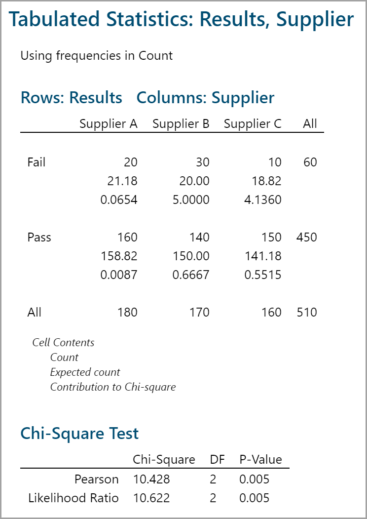
The image below shows a typical output from statistical software like Minitab. Notice how it provides the observed count, the expected count, and the contribution of each cell to the overall Chi-Square statistic. This makes it easy to spot the cells with the largest discrepancies.

Conclusion

You have now added another essential hypothesis test to your toolkit. While t-tests and ANOVA are your go-to tools for continuous data, the Chi-Square test is your primary method for analyzing attribute or categorical data. It provides a structured way to determine if a relationship exists between two categorical factors, such as defect types, production lines, suppliers, or inspection results.

Key Takeaways:

• The Chi-Square Test of Independence is used to determine if there is a statistically significant association between two categorical variables.
• The test works by comparing observed counts in a contingency table to the expected counts that would occur if the variables were independent.
• The decision is based on the p-value: if p < 0.05, you reject the null hypothesis and conclude that the variables are related.
• A significant result is just the start. The real value comes from interpreting the result by comparing observed vs. expected counts to understand the nature of the relationship and guide your root cause analysis.

Preview of the Next Lesson:

So far in this module, we have covered hypothesis tests that involve at least one categorical variable (t-tests, ANOVA, and Chi-Square). In our next module, we will shift our focus to exploring the relationship between two continuous variables. We will begin by learning how to visualize this relationship using scatter plots and quantify its strength with the correlation coefficient, which are the first steps into the world of regression analysis.