Introduction
Welcome back! In our last lesson, we mastered the use of t-tests to compare the means of one or two groups. We confirmed that these tests are essential for verifying if a change has had a statistically significant impact, or if two suppliers are performing differently. However, we ended with a critical question: what tool should we use when we need to compare three or more groups, like the performance of three different production shifts or four different machines?
Attempting to answer this by running multiple two-sample t-tests (e.g., Shift A vs. B, A vs. C, and B vs. C) is a common mistake. Each test has a chance of a false positive (a Type I error), and as you run more tests, the overall probability of making such an error inflates dramatically.
This is where Analysis of Variance (ANOVA) comes in. This lesson addresses the learning outcome: Conduct ANOVA to compare means across multiple groups (e.g., machines, shifts, suppliers). We'll explore how ANOVA provides a single, robust test to determine if there's a significant difference somewhere among your groups, maintaining a controlled error rate. This is a cornerstone of the Analyze phase in DMAIC, allowing you to efficiently test multiple potential root causes at once.
The Core Idea: Analyzing Variance to Compare Means
The name "Analysis of Variance" can seem counterintuitive since our goal is to compare means. The genius of ANOVA is that it assesses the difference between group means by analyzing their variances.
Imagine you have data from three different machines. ANOVA answers the question: "Is the variation between the average performance of these machines significantly greater than the natural, random variation we see within each machine's own performance?"
- Within-Group Variation (or "Error"): This is the inherent, random noise or variability of the process. For example, not every part produced by Machine A will be identical.
- Between-Group Variation (or "Treatment"): This is the variation caused by the different groups or "factors" you are testing (the different machines).
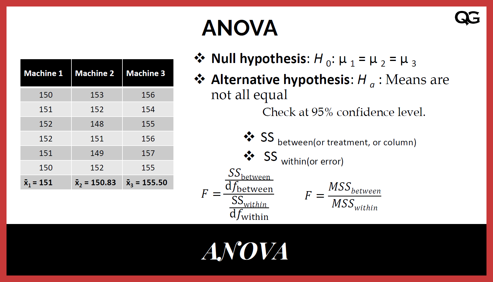
The test statistic for ANOVA is the F-statistic (or F-ratio):
- If the F-statistic is close to 1, it means the variation between the groups is about the same as the random variation within the groups. We would conclude the group means are not significantly different.
- If the F-statistic is much larger than 1, it indicates that the differences between the group means are large compared to the random noise. This suggests that at least one group is truly different from the others.
Let's watch a short video that explains this fundamental concept.
ANOVA (Analysis of Variance) Analysis – FULLY EXPLAINED!!!
This clip from the Green Belt Academy video "ANOVA (Analysis of Variance) Analysis – FULLY EXPLAINED!!!" explains why we analyze variance to draw conclusions about means.
Please watch from 01:45 to 02:32. The key takeaway is understanding that ANOVA works by creating two different estimates of variance and comparing them.
One-Way ANOVA: Comparing Groups for a Single Factor
The most common type of ANOVA is the One-Way ANOVA, used when you are testing one categorical factor with three or more "levels" (groups).
- Factor: The variable you are investigating (e.g., Supplier).
- Levels: The different groups within that factor (e.g., Supplier A, Supplier B, Supplier C).
- Response: The continuous measurement you are analyzing (e.g., material hardness, part diameter).
Hypotheses for One-Way ANOVA
The hypotheses are always structured as follows:
- Null Hypothesis (H₀): All group means are equal. (e.g., μ_supplierA = μ_supplierB = μ_supplierC)
- Alternative Hypothesis (H₁): At least one group mean is different.
It's crucial to note that ANOVA's p-value only tells you if there is a difference somewhere, not which specific group or groups are different.
A Practical Manufacturing Example
Let's consider a scenario from a real Six Sigma project described in the paper "Implementation of Six Sigma in a Manufacturing Process" (LINK). The team needed to determine if there was a performance difference across four operational shifts (Shifts A, B, C, and D).
The Question: Is the average efficiency the same across all four shifts?
Steps:
- State the Hypotheses:
- H₀: The mean efficiency of all four shifts is equal (μ_A = μ_B = μ_C = μ_D).
- H₁: The mean efficiency of at least one shift is different from the others.
- Check Assumptions:
- Independence: Samples from each shift are independent.
- Normality: The data for each shift is approximately normally distributed.
- Equal Variance: The variance of the data within each shift is roughly equal (checked with Levene's or Bartlett's test in statistical software).
- Perform the Test and Interpret the ANOVA Table:
You would use statistical software (like Minitab or even Excel) to run the analysis. The output is a standard ANOVA table. Let's break down what each column means using a generic example.
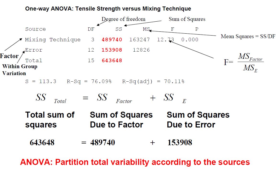
Key Columns to Interpret:
- F (F-statistic): The calculated ratio of
MS (Factor)/MS (Error). - P (p-value): The probability of observing an F-statistic this large or larger if the null hypothesis were true.
The Decision Rule:
Just like with t-tests, if p-value < 0.05, you reject the null hypothesis. You have sufficient evidence to conclude that not all group means are equal.
In the shift performance example from the paper, the p-value was 0.000. This is less than 0.05, so the team correctly rejected the null hypothesis and concluded that there is a significant difference in efficiency among the four shifts.
After ANOVA: Finding the Specific Difference with Post-Hoc Tests
So, we know at least one shift is different, but which one? To find out, we use a post-hoc test (meaning "after this"). The most common one is Tukey's Honest Significant Difference (HSD) test.
This test compares all possible pairs of means (A vs. B, A vs. C, A vs. D, B vs. C, etc.) and tells you which specific pairs are significantly different from each other. In the shift example, the analysis showed that Shift A had a significantly better performance, while Shift D had the lowest. This allowed the team to focus their efforts on standardizing the best practices from Shift A across the other shifts.
Let's dive deeper into the mechanics and logic of a full One-Way ANOVA.
ANOVA (Analysis of Variance) Analysis – FULLY EXPLAINED!!!
This video from Green Belt Academy will walk us through a complete ANOVA example, from setting up the problem to calculating the F-value and making a decision. This will formalize the concepts we've just discussed.
Please watch the following segments: Setting up the Example (03:07 - 05:11): This introduces the terminology and a practical example comparing horsepower at different octane levels. Defining the Hypotheses (05:11 - 07:49): Pay close attention to how the null and alternative hypotheses are framed for ANOVA. Making the Decision (24:25 - 28:49): This part shows how the calculated F-value is compared against a critical value (or how you would use a p-value) to make a final accept/reject decision. Focus on the logic of the decision, not on memorizing the manual calculations.
A Glimpse into Advanced Analysis: Multi-Factor (Two-Way) ANOVA
As you advance toward a Black Belt level, you'll encounter situations where more than one factor might be influencing your process. A Two-Way ANOVA allows you to test two factors simultaneously.
Manufacturing Scenario:
A medical device manufacturer is seeing defects in molded parts. They suspect both the shift (Day, Swing, Night) and the material lot (Lot A, Lot B) could be causes.
A Two-Way ANOVA not only tells you if Shift has an effect and if Material Lot has an effect (these are called main effects), but it also reveals if there is an interaction effect between them.
An interaction means the effect of one factor depends on the level of the other factor. For example, an interaction would exist if the Night shift only produces high defects when using Material Lot B. This is an incredibly powerful insight that running two separate One-Way ANOVAs would completely miss.
This video from Oxford Academic demonstrates a multi-factor ANOVA in Minitab. We'll focus on the second part, which clearly shows how to analyze and interpret a significant interaction.
Please watch from 04:07 to 07:54. Focus on these key points: Notice that the P-value for the interaction term (Temp*Catalyst) is significant (0.030). Look at the interaction plot at the end. See how the lines are not parallel? This is the visual sign of an interaction. The effect of temperature is different for Catalyst C7 than it is for Catalyst C6.
This concept of interactions is fundamental to more advanced process optimization and Design of Experiments (DOE), which we will cover later in the course.
Conclusion
In this lesson, we've added a powerful statistical tool to your analytical arsenal. You now understand how to move beyond simple two-group comparisons and analyze the impact of multiple machines, suppliers, shifts, or other categorical variables on your process output.
Key Takeaways:
- ANOVA is used to compare the means of three or more groups by analyzing their variances.
- The F-statistic is the ratio of variation between groups to the variation within groups. A large F-value suggests a significant difference in means.
- A p-value < 0.05 in an ANOVA test indicates that at least one group mean is different, but it doesn't specify which one.
- Post-hoc tests like Tukey's HSD are used after a significant ANOVA result to identify which specific pairs of means are different.
- Two-Way ANOVA allows for the analysis of two factors and, critically, the interaction between them.
Preview of the Next Lesson:
ANOVA is the perfect tool for understanding how categorical factors (like Machine A, B, or C) affect a process mean. But what if your input variable is continuous, such as temperature, pressure, or time? In our next lesson, we will begin exploring regression analysis, which allows us to visualize and model the relationship between continuous variables.