Scatter Plots and Correlation

Visualizing Relationships with Scatter Plots

The first step in understanding the relationship between two continuous variables is always to visualize the data. The primary tool for this is the scatter plot (also called a scatter diagram).

A scatter plot displays pairs of data on a two-dimensional graph. In a Six Sigma context, we typically plot:

• The Independent Variable (X) on the horizontal x-axis. This is the variable we suspect is a cause or a process input (e.g., machine setting, temperature, pressure).
• The Dependent Variable (Y) on the vertical y-axis. This is the effect or the process output we are measuring (e.g., a quality characteristic, defect rate, cycle time).

By plotting these pairs of (X, Y) data, we can visually inspect the resulting pattern to see if a relationship exists.

Creating and Interpreting a Scatter Plot

Creating a scatter plot is straightforward, and modern software makes it simple. However, understanding the steps and what to look for is key. Let's walk through a practical manufacturing example.

Scenario: A pharmaceutical company is experiencing variation in the hardness of its tablets. The team hypothesizes that the compression force applied during manufacturing is a key driver of this variation.

To test this, they collect paired data for 25 batches: the Compression Force (X) and the resulting Tablet Hardness (Y).

As the example shows, the pattern of the plotted points reveals the nature of the relationship. There are three main types of linear relationships you can identify:

1. Positive Correlation: As X increases, Y tends to increase. The points form a pattern that trends upward from left to right. The tablet hardness example shows a clear positive correlation.
2. Negative Correlation: As X increases, Y tends to decrease. The points form a pattern that trends downward from left to right. For example, you might find that as operator training hours increase, the number of defects decreases.
3. No Correlation: The points appear randomly scattered with no discernible trend. This is also a valuable finding, as it suggests the input variable (X) does not have a significant linear relationship with the output variable (Y).

It's also possible to see non-linear relationships (e.g., a U-shaped curve), where the relationship changes direction.

Quantifying the Relationship: The Correlation Coefficient (r)

Visual inspection is powerful, but it's subjective. To objectively measure the strength and direction of the linear relationship between two continuous variables, we calculate the Pearson Correlation Coefficient, denoted as $r$.

The correlation coefficient is a single number that summarizes the scatter plot:

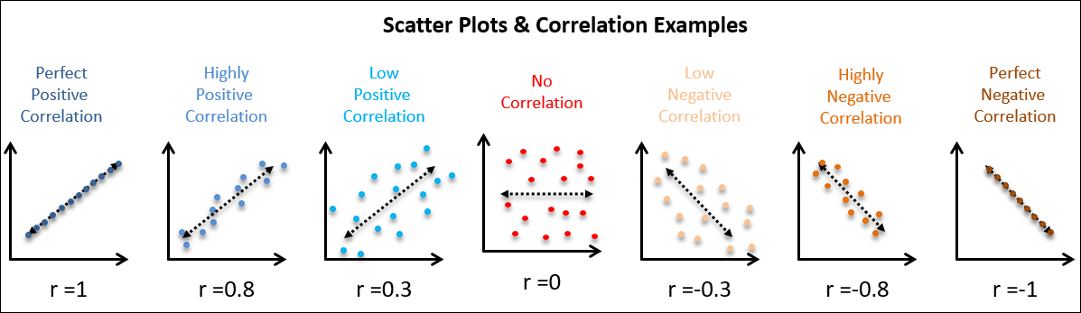
• It ranges from -1 to +1.
• The sign (+ or -) indicates the direction of the relationship (positive or negative).
• The magnitude (how close the value is to 1 or -1) indicates the strength of the linear relationship.

The image below gives you a clear visual guide for how the appearance of the scatter plot corresponds to different values of $r$.

Interpreting the Strength of Correlation

So, how do you decide if a correlation is "strong" or "weak"? While context is important, there are some common rules of thumb used in practice.

In a manufacturing setting, discovering even a moderate correlation (e.g., $|r|>0.5$) between a process setting and a quality outcome is often a significant finding that warrants further investigation.

A Critical Warning: Correlation is Not Causation

This is one of the most important principles in data analysis. Just because two variables are strongly correlated does not automatically mean that one causes the other.

The video you watched made this point, and it's worth repeating. A strong correlation might exist for several reasons:

1. Direct Causation: X does indeed cause Y. (e.g., Increased compression force causes increased tablet hardness).
2. Reverse Causation: Y causes X.
3. Confounding Variable: A third, unmeasured variable (Z) is causing both X and Y to change. The classic example is the strong positive correlation between ice cream sales (X) and shark attacks (Y). The lurking variable is hot weather (Z), which causes more people to buy ice cream and more people to go swimming.

As a practitioner, your job is to use your process knowledge combined with statistical evidence. A scatter plot and correlation give you a clue—a hypothesis that a relationship exists. Further analysis, like Design of Experiments (DOE), is often needed to prove causation.

Putting It All Together: From Data to Insight

When analyzing a process, you often have multiple potential input variables (X's) that might affect your output (Y). A correlation matrix (or a scatter plot matrix) is an efficient way to visualize the relationships between all pairs of variables at once.

This technique is extremely useful in the early stages of the Analyze phase to screen a large number of potential X's and decide which ones to investigate more deeply.

Conclusion

In this lesson, we established the foundational techniques for exploring relationships between continuous variables. You've learned how to use a simple graphical tool, the scatter plot, to gain immediate visual insights and how to back that up with a quantitative measure, the correlation coefficient.

Key Takeaways:

• Scatter plots are your first step to visually assess the relationship between a continuous input (X) and a continuous output (Y).
• The plot's pattern reveals the direction (positive, negative) and gives a sense of the strength of the relationship.
• The correlation coefficient (r) provides a numerical value from -1 to +1 that quantifies the strength and direction of the linear relationship.
• Always remember the critical rule: correlation does not imply causation. A strong correlation is a signal to investigate further, not a final conclusion about cause and effect.

Preview of the Next Lesson:

Visualizing and quantifying a relationship is a great start, but what if we want to create a predictive model? If a strong linear relationship exists, we can describe it with a mathematical equation. In the next lesson, we will do just that by learning how to build and interpret a simple linear regression model, turning our scatter plot into a powerful predictive tool.