Introduction
Welcome to the next lesson in our Design of Experiments (DOE) module. In our previous session, we meticulously covered how to design factorial experiments and, crucially, how to evaluate their limitations by examining the design resolution and alias structure. You learned that the efficiency of fractional factorial designs comes with a trade-off: confounding, where the effects of certain factors or interactions become entangled.
Now that we have designed a statistically sound experiment, it's time to move to the next step in the DMAIC process: Analyze. We will assume the experiment has been run and the data collected. Our goal today is to answer the core question of any experiment: Which factors actually matter?
This lesson addresses the learning outcome: Analyze factorial experiment results using ANOVA to determine factor significance. We will introduce Analysis of Variance (ANOVA) as the statistical engine that powers DOE analysis. You will learn how to interpret the standard output from an ANOVA to confidently declare which factors and interactions have a statistically significant impact on your process response.
1. The Core Logic of ANOVA
At its heart, ANOVA is a hypothesis testing tool. For any given factor in your experiment (e.g., Temperature), the null hypothesis () is that the factor has no effect on the response variable (e.g., coating thickness). The alternative hypothesis () is that it does have an effect.
But how does it decide? ANOVA works by partitioning the total variation in your experimental data. It compares the variation caused by changing a factor's levels (the "signal") to the natural, random variation that exists within each level (the "noise" or "error").
If the signal is strong relative to the noise, we reject the null hypothesis and conclude the factor is significant. This comparison is quantified by the F-statistic (or F-value).
To build a solid intuition for this, let's watch a video that breaks down the fundamentals of ANOVA.
ANOVA (Analysis of Variance) Analysis – FULLY EXPLAINED!!!
This video from Green Belt Academy provides an excellent, step-by-step explanation of the core concepts behind ANOVA. It uses a simple one-factor example, which is the perfect foundation before we apply it to a multi-factor experiment.
Please watch the following segments. Focus on understanding the 'why' behind the calculations. Null and Alternative Hypothesis (05:11 - 08:01): Pay close attention to how the null hypothesis (all mean values are equal) is stated. This section introduces the F-value as the tool we use to make a decision. Mean Square as Variance (08:01 - 10:43): This is a critical concept. Understand that the 'Mean Square' (MS) in an ANOVA table is an estimate of variance. The F-value is a ratio of two variances. Between vs. Within Variation (10:43 - 18:40): This is the most important part of the video. It masterfully explains how ANOVA compares the variation between treatment groups (MS Treatment) to the variation within treatment groups (MS Error). A large F-value occurs when the variation between groups is much larger than the variation within them, indicating a significant effect.
As the video explained, the F-value is calculated as:
A large F-value tells us the variation caused by changing our factor's settings is significantly greater than the background noise of the process.
2. Deconstructing the ANOVA Table
Statistical software packages present the results of this analysis in a standardized format called an ANOVA table. Understanding this table is the key to interpreting your experimental results.
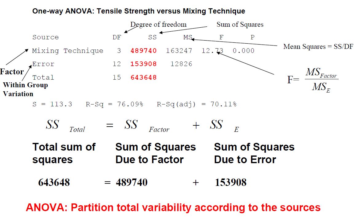
Let's break down the key columns you will always see in an ANOVA table for a factorial experiment:
- Source: Lists the potential sources of variation: each main factor, each interaction, and the error.
- DF (Degrees of Freedom): An indicator of how much information is available to estimate each source of variation. For a factor, it's the number of levels minus 1.
- SS (Sum of Squares): The magnitude of variation accounted for by that source.
- MS (Mean Square): The variance for that source, calculated as .
- F-Value: The test statistic calculated for that source ().
- P-Value: This is your primary decision-making tool. It represents the probability of seeing an F-value as large as the one calculated if the null hypothesis (no effect) were true.
The Decision Rule: If the P-value for a source is less than your chosen significance level (alpha, ), you reject the null hypothesis. In most industrial settings, is set to 0.05.
In short: P < 0.05 means the factor or interaction is statistically significant.
3. Case Study: Analyzing a Factorial Experiment
Let's apply this to a practical manufacturing scenario. Imagine you are developing a new insulation product and want to understand what drives its physical strength. You've run a factorial experiment with four factors.
Example of Analyze Factorial Design
This Minitab support article provides a perfect example of a factorial analysis. It walks through a scenario and the interpretation of the resulting ANOVA table, which is exactly the skill we are focused on.
Please read through this example, focusing on two key parts: The Scenario: Read the introductory paragraph to understand the goal: analyze how material type, injection pressure, injection temperature, and cooling temperature affect insulation strength. The Analysis of Variance Table: Locate the table under the 'Analysis of Variance' heading. Using the P-value column and the decision rule (P < 0.05), identify which factors are significant. Compare your conclusion to the text in the 'Interpret the results' section.
From the example, you should have observed the following in the ANOVA table:
| Source | P-Value | Significant? (at ) |
|---|---|---|
| Material | 0.017 | Yes |
| InjPress | 0.002 | Yes |
| InjTemp | 0.005 | Yes |
| CoolTemp | 0.015 | Yes |
| 2-Way Interactions | 0.366 | No |
The analysis is clear: all four main factors have a significant effect on the insulation's strength. Furthermore, the overall p-value for the "2-Way Interactions" block is 0.366, indicating that there are no significant interactions between these factors. This is a straightforward result where we can focus on understanding and optimizing each of the main factors independently.
4. The Critical Role of Interactions
In the previous example, things were simple. But often, factors do not act independently. The effect of one factor can change depending on the level of another. This is an interaction, and failing to identify it is a major risk in process improvement. ANOVA is the tool that allows us to statistically confirm these interactions.
Let's look at another manufacturing case study, this time involving a coating process.
This second Minitab example illustrates a more complex, and more realistic, situation where an interaction effect is highly significant. This highlights a critical rule of DOE analysis.
First, find the 'Analysis of Variance for Thickness' table. Examine the P-values for all sources, including main effects (Time, Setting) and interactions (Time*Setting). Identify all significant terms. Now, read the 'Interpret the results' section carefully. Pay special attention to the paragraph that begins 'Time*Setting is an interaction effect...'. It explains the most important rule when interpreting results with significant interactions.
In this coating experiment, the ANOVA table shows that the Setting factor is significant (P=0.001), but crucially, the Time*Setting interaction is also significant (P=0.002).
As the resource explains, this means you should not interpret the main effect of Setting in isolation. The effect of the machine setting on coating thickness depends on the time of day (morning vs. evening). The means table in the example shows this clearly:
- With a setting of 44, time 2 (evening) gives a thicker coating.
- With a setting of 52, time 1 (morning) gives a thicker coating.
If you had only looked at the main effect of Setting, you might have concluded that "Setting 52 is best" because it has the highest average thickness overall. But the interaction tells you the real story is more nuanced. This is a profound insight that would be missed without testing for interactions, and it is a hallmark of a properly executed Six Sigma project.
Conclusion
Today you have learned how to use Analysis of Variance (ANOVA) to move from raw experimental data to confident conclusions about your process. This is the statistical engine that drives the Analyze phase of any DOE project.
Key Takeaways:
- ANOVA partitions variation to determine if the "signal" from a factor is stronger than the background "noise" of the process.
- The ANOVA table is the standard output, and the P-value is your key decision-making metric. A P-value less than 0.05 indicates a factor or interaction is statistically significant.
- Always analyze interaction effects first. If an interaction (e.g., A*B) is significant, the main effects involved (A and B) cannot be interpreted on their own. Their effect on the response is interdependent.
Preview of the Next Lesson:
We can now statistically declare which factors and interactions are significant. But ANOVA tables don't tell the whole story. They don't tell us the direction or magnitude of the effects, nor do they help us visualize complex interactions.
In our next lesson, we will focus on the graphical tools that bring your results to life. We will learn how to "Interpret main effects and interaction plots to understand the behavior of process factors." These plots are essential for communicating your findings and making practical decisions about how to optimize your process.